Basis function coefficients

[Rebecka N]

Any complex periodic wave can be represented as a sum of weighted basis functions. The basis functions are orthogonal, meaning they have the same amplitude but are multiples of the lowest frequency sinusoid of the set. The question is how to find the coefficients / weights for these basis functions. The video explained that you take the sinusoid you want to weight and multiply it with the original wave. The product of this operation will be large for sinusoids which are similar to the original wave whereas it will be small for dissimilar sinusoids. This makes intuitive sense as you’d want to add more of the very similar basis functions than you’d want to add of the dissimilar ones when you add up sinusoids to create your complex wave.

I can’t quite visualize how this multiplication is performed, however. These are my follow-up questions:

a) Is it the case that you are able to find the coefficients of the basis functions through multiplication because of symmetry reasons? If you look at my drawing I have tried to visualize what I imagine is happening. The two plots on the bottom are supposed to show the same wave, ie “what would happen if we multiplied two identical waves together?”. We would do 1×1 at the first sampling point and -1x-1 at the second sampling point. The sum would be 2. Conversely, the diagram at the top shows what happens if we multiply two dissimilar waves together. At the first sampling point we get 1×0.75 and at the second point we get -1×0.75 and therefore end up with the sum of 0. In other words, we get cancelling effects for dissimilar waves because the amplitude of one will be positive whereas the amplitude of the other will be negative at certain points in time and we therefore get some negative products when we perform this step-wise multiplication. These cancelling effects are the same phenomenon that makes the basis functions orthogonal because if you would perform this multiplication on any pair of basis functions – instead of a basis function and the composite wave – they would cancel each other out completely?
Does my description make sense? Have I understood what you meant in the video?

b) If the above is correct, is this why I see so many explanations on YouTube involving proofs with integrals? Because performing this step-wise multiplication at each point of the curves and adding the products together is like integrating: dx is the distance you travel along the x-axis (stepping through each sample-point along the time axis) and the y-values are the products of the two curves for that point?

c) What about the actual number we end up with: it is big when the waves match and small when the waves are different. Wouldn’t we end up with 1 as a coefficient if the waves were identical? So presumably “a big number when the waves are similar” means a fraction that is close to 1? If so, then the effect of cancellation described above must be such that we always end up with coefficients like 0 <= c <= 1, regardless of the amplitudes on the y-axis. I.e. in my example we get 2 as the coefficient a0 when we add the identical waves because we imagine that the amplitudes were 1 and -1 at the sampling points but presumably it doesn’t matter what we get as the sum for two points on these curves because multiplication at EVERY single point along these curves will eventually give us a coefficient that is between 0 and 1? (… though I’m thinking that multiplication at every point would amount to multiplication of an infinite series because the waves are continuous and that maybe this is why we get irrational numbers like Catherine showed us in the live session today… ? … but perhaps that is something we’ll get into later in the course).

Attachments:

You must be logged in to view attached files.

[Catherine Lai]

Any complex periodic wave can be represented as a sum of weighted basis functions. The basis functions are orthogonal, meaning they have the same amplitude but are multiples of the lowest frequency sinusoid of the set. The question is how to find the coefficients / weights for these basis functions. The video explained that you take the sinusoid you want to weight and multiply it with the original wave. The product of this operation will be large for sinusoids which are similar to the original wave whereas it will be small for dissimilar sinusoids. This makes intuitive sense as you’d want to add more of the very similar basis functions than you’d want to add of the dissimilar ones when you add up sinusoids to create your complex wave.

We need to first clarify what “orthogonal” means here. The fact that the basis functions are orthogonal means that if you measure the similarity between the functions using a dot (aka inner) product (as we do in the DFT), the similarity will be zero. The fact that the sinusoids are multiples of the the lower frequency one guarantees this orthogonality property when we are dealing with discrete (i.e., sampled sinusoids) rather than continuous ones. This is what allows us to pick out the presence of specific frequencies with the DFT. When we do the dot product between the input and a specific basis sinusoid, we’re basically zeroing out all the frequencies and so just seeing how much of that basis sinusoid frequency is in the original signal.

To think about why the dot product works as a measure of similarity, we need to think about the sampled sinusoids as vectors. Each of the basis sinusoids consists of N samples (corresponding to the number of samples in the input window). This means we can think of each of the sinusoids as an N dimensional vector.
For example, let’s call the first basis sinusoid s1. The DFT represents this with N samples so s1 = [u1, u2,….,uN], where u1,..,uN represent the sampled amplitudes of that sinusoid in time. Similarly we can take second basis sinusoid as s2=[v1,v2,….,vN]. As sine waves they look like this:

To calculate the dot product between s1 and s2 we first take the pairwise multiplication at each dimension of the vector, then sum all of those values together:
u1*v1+u2*v2+…+uN*Vn. So this gives us one number with corresponds to a how much the two vectors were pointing in the same direction. If this value is zero we intepret this geometrically as the vectors being orthogonal (i.e. perpendicular). Intuitively, you can think of this as meaning there is no correlation between the two vectors. This is a nice video that explains dot products and their geometric interpretation.

For the DFT the dot product is taken between the sampled input: x = [x1,…,xN] and each of the basis vectors s_k = [a1,….,aN].

So DFT[k] = x1*a1 + ….+ xN*aN.

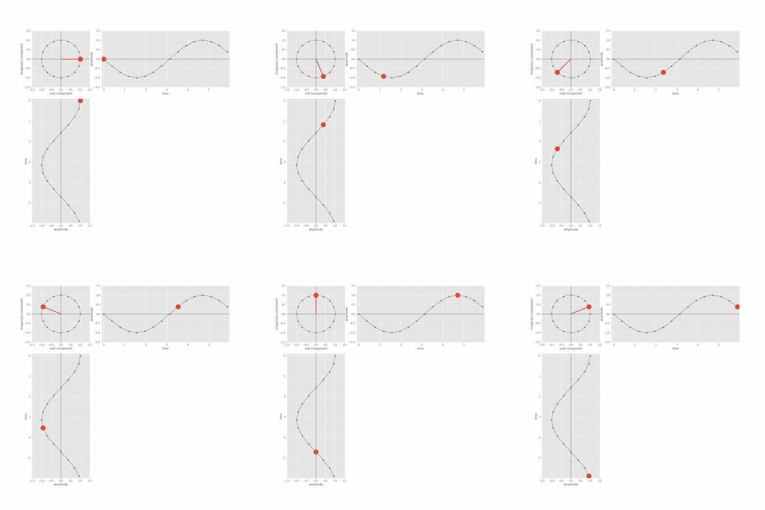
From this we can derive the magnitude (scale) and phase (shift) coefficients associated with different basis sinusoid frequencies. We just focused on magnitude in the lecture, but you can get the phase out of the result of the dot product too because the actual DFT dot product involves complex sinusoids (in the sense of complex numbers, a+jb with j=sqrt(-1)) not just real valued sine waves. There’s more detail on this Module 3 lab notebooks (more in the extension notebooks), but the general idea is that the DFT is actually taking the dot product between the (real valued) [x1,…,xN] and a complex sinusoid which we can in turn think of in terms of separate cosine and sine waves of a specific frequency. The following git shows the complex sinusuoid (cycles of the circle top left), and the relation to sine (top right) and cosine functions (bottom left).

[to be continued!…]

[Catherine Lai]

Is it the case that you are able to find the coefficients of the basis functions through multiplication because of symmetry reasons? If you look at my drawing I have tried to visualize what I imagine is happening. The two plots on the bottom are supposed to show the same wave, ie “what would happen if we multiplied two identical waves together?”. We would do 1×1 at the first sampling point and -1x-1 at the second sampling point. The sum would be 2. Conversely, the diagram at the top shows what happens if we multiply two dissimilar waves together. At the first sampling point we get 1×0.75 and at the second point we get -1×0.75 and therefore end up with the sum of 0. In other words, we get cancelling effects for dissimilar waves because the amplitude of one will be positive whereas the amplitude of the other will be negative at certain points in time and we therefore get some negative products when we perform this step-wise multiplication. These cancelling effects are the same phenomenon that makes the basis functions orthogonal because if you would perform this multiplication on any pair of basis functions – instead of a basis function and the composite wave – they would cancel each other out completely?Does my description make sense? Have I understood what you meant in the video?

There are a few different things going on here:

1. You can find the DFT coefficients (i.e. the DFT outputs) by performing the dot product.
2. You can see that the dot product between DFT basis sinusoids will be zero because of symmetry of sinusoids around the x-axis of a time versus amplitude plot.

First let’s consider
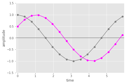
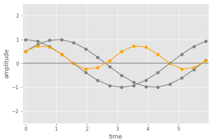
– an input 16 samples of 1 period of a cosine wave with a small phase shift (magenta)
– 16 samples of a cosine wave of the same frequency (hence period) but without the phase shift (this is equivalent to the 1st DFT basis sinusoid) (grey).

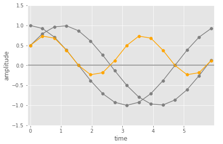
This next figure we see those two cosine wave, and the pairwise multiplication of the samples of those two waves (in orange).

Here you can see that the orange values are mostly above zero amplitude and the positive values have larger absolute values than the negative ones. When you add them up (as the last part of the dot product) you would get a non zero value (positive in this case). You can think of this as the average value of the multiplication points being above zero.

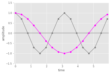
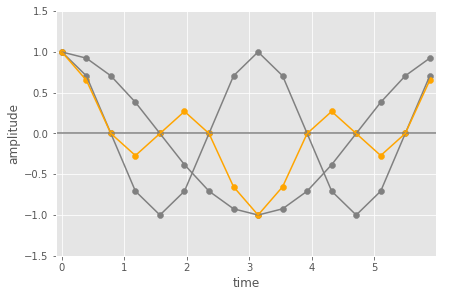
Now let’s look at the case where we the input is the 1st DFT basis sinusoid and we take the dot product with the 2nd DFT basis sinusoid (so twice the frequency of the 1st DFT basis sinusoids – 2 cycles in the same time window).

In this case, the pairwise multiplication results in values that are symmetric around zero amplitude. Over the period the average of the orange points will be zero (because the positive points are in in effect cancelled out by the negative ones).

You now might also think about this in terms of overall area under the curve being zero! But remember we don’t actually have a curve here, just the sampled points!

However, this links to the point (b) about integrals. Yes, it’s basically the same thing but since we are working in a discrete space we need to take sums instead of integrals. When dealing with continuous functions we use the Continuous Fourier Transform which takes the integral instead of the sum. The difference is that we have a limit of what dx can be (determined by the sampling rate) so we can’t make dx infinitely small as is required for an integral (but it’s the same concept). Instead we multiply the discrete samples that are aligned in time and sum them up.

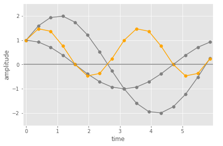
For point (c), Note that the dot product isn’t scaled, so it can be bigger than 1. The magnitude shown on the spectrum for a detected frequency will be proportional to the amplitude of that frequency in the input. You can see this in the figures below.

The first shows the same as above (same frequency with a phase shift) versus a version where the input has double the peak amplitude. The positive values in the pairwise multiplication (orange) are bigger, so the overall dot product (sum) value will be too.

Some these details are definitely easier to see if you go through the actual mechanics of the DFT equation. We’ve set the mathematical details as beyond the examinable scope of this course, but you can find some more detail on this in the Module 3 lab notebooks, specifically notebook 3 (“discrete Fourier Transform in detail”). This is marked as extension material but it still might be useful to play with the visualisation of the dot product at the end of the notebook.

[Author]

Posts