[Simon]

Maths looks fine on Chrome for iOS

[Simon]

Yes, that’s correct. Gain is simply a technical term for the amount by which a signal is multiplied.

[Simon]

Vocal tract length

On average, men have slightly longer vocal tracts than women, and so the formants in male speech will be a little lower than in female speech.

Fundamental frequency

Generally, male speech has a lower fundamental frequency (F0). This is due to a combination of anatomical differences, both in the vocal folds themselves and the larynx. This article seems to summarise the factors quite well.

[Simon]

For this course, you do not need to be able to state or derive formally what the computational complexity of algorithms is, although you should understand informally that some algorithms are more complex (i.e., require a larger number of computations) than others.

Nevertheless, it’s still useful to understand computational complexity. Let’s just keep things informal here and only mention the most important case, and that is the complexity of a CART when we are using it at ‘run time’:

Computational complexity of using a CART to classify an unseen data point

This depends on the depth of the tree, because that determines how many questions you need to ask about the predictors. The depth of the tree is proportional to the logarithm (to base 2) of the number of leaves. This is very nice: the logarithm of a number grows slowly as that number gets larger. So, even trees with very large numbers of leaves will not be very deep. For example, a tree with 1000 leaves will only have a depth of around 10. That makes CARTs very fast to use: asking 10 binary questions about predictors will be computationally very fast.

What is the depth of a tree?

This is the number of edges (the edges join up the nodes) from the root to a leaf. The depth might vary in different parts of the tree, of course.

[Simon]

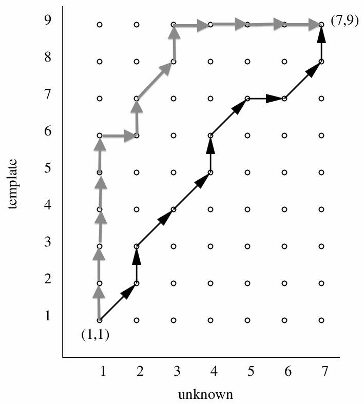
Think about the grid, which is the data structure used for Dynamic Time Warping. Paths from one corner to the diagonally-opposite corner must pass through the points on the grid, summing up local distances as they go. Paths close to the main diagonal generally pass through fewer points in total than paths that stray far away from the main diagonal.

You can see in the diagram above how the two paths differ in the number of local distances that they must sum up. This leads to a bias in favour of paths that stay close the the main diagonal.

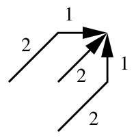
To reduce this bias, lots of solutions were proposed back at the time when DTW was the state-of-the-art. One is to penalise diagonal paths (e.g., add a penalty cost to the distance-so-far every time a diagonal move is made). One popular method was to impose local constraints, such as in this diagram (the numbers are weights or penalty terms):

Is this still important?

For automatic speech recognition, this is all outdated and no longer important. But there is a general lesson that might apply to other applications of dynamic programming: look for biases towards certain solutions, and ask whether that needs to be compensated for.

[Simon]

You’re mixing up two distinct processes.

Warping the frequency scale

There are a variety of perceptually-motivated frequency scales, and we could choose any of them (Mel, Bark, ERB, …). They all have something in common, and that is that they are non-linear. This non-linearity might or might not be implemented as a logarithm, but note that we are not taking the logarithm of the energy of the speech signal, we are just warping the frequency scale. Think of it as stretching the vertical axis in a spectrogram so that the lower frequencies occupy more of the scale, and that higher frequencies are squashed into less of the scale.

Taking logarithms of filterbank outputs

Here is where taking logs is crucial: this is the point at which we convert a multiplication in the frequency domain (the source spectrum has been multiplied by the vocal tract frequency response) into an addition (a sum) in the cepstral domain.

After that multiplication-to-addition conversion, then we can split the source and frequency contributions to the sum. This is possible because their contributions are at different quefrencies. By using a cosine series expansion, we spread these contributions out along the quefrency scale and can then – for example – ignore those parts that relate to the source.

[Simon]

HInit performs uniform segmentation, immediately followed by Viterbi training. The output that you are seeing for several iterations is for the Viterbi stage of training.

[Simon]

Next, let’s write a script that calls another script, and passes a value to it on the command line. Here are the two scripts:

#!/bin/bash

MYVARIABLE=$1

echo "This is the child script and the value passed was" ${MYVARIABLE}

and

#!/bin/bash

# this is the parent script

echo "This is the parent script and it is about to run the child script three times"

./scripts/child.sh one
./scripts/child.sh two
./scripts/child.sh three

echo "Now we are back in the parent script"

echo "Let's get smarter and write code that is easier to maintain"

for COUNT in one two three
do
	./scripts/child.sh $COUNT
done

echo "Pretty nice - but we can do even better and read in the list from a file"

for FRUIT in `cat lists/fruit_list.txt`
do
	./scripts/child.sh ${FRUIT}
done


echo "Much better. Now let's save the output to a file so we can inspect it later"
echo "This method will overwrite the contents of the file, if it already exists"

(for FRUIT in `cat lists/fruit_list.txt`
do
	./scripts/child.sh ${FRUIT}
done) > output.txt


echo "Another way is to append lines to an existing file"

echo "This line will appear in the file" >> output.txt


for FRUIT in `cat lists/fruit_list.txt`
do
	./scripts/child.sh ${FRUIT}  >> output.txt
done

echo "Now you need to look at the file just created, called output.txt"

echo "For example, you could now type 'cat output.txt' or open it in Aquamacs"

and the file fruit_list.txt contains

apples
bananas
pears
oranges

now let’s run it

$ ./scripts/parent.sh 

I’ve attached a zip file containing everything you need.

Attachments:

You must be logged in to view attached files.

[Simon]

Once per utterance to be recognised.

I think this topic could help – read it through, then post any follow up questions there.

The key idea is that the language model and the acoustic models (HMMs) have been compiled together and therefore are just one big HMM. Token passing is performed on that.

[Simon]

Put this line

set -x

somewhere near the start of your script. It will cause the complete HVite command line to be printed just before it is executed. That will help you see what is wrong with the arguments you are passing to HVite.

The shell is trying to execute “resources/word_list_seq” which obviously should never happen – you might have a space after one of the “\”, or blank lines or comments in the middle of the HVite command, perhaps.

[Simon]

Next time I have a wet Sunday afternoon with nothing better to do, I may indeed do a longer animation for connected word token passing. Don’t hold your breath though.

Yes – you seem to have got it: tokens that have “looped back” from the final state of one word model to the initial state of another (or indeed the same) word model will simply compete with whatever tokens is encounters there. The mechanism is exactly the same as tokens meeting within words.

Tokens will need to remember which words they have been through, so that we can read the most likely word sequence off the winning token. Appending a word label to a token’s internal word link record every time it leaves a word model is the way to do that, yes.

[Simon]

Pruning is a separate issue.

[Simon]

Don’t think of lots of HMMs running in parallel. Think of the compiled network as one big HMM. That’s because it really is just one big HMM.

It just happens to have a more interesting topology than the individual left-to-right word models, but that makes no difference to token passing. There’s still a start state, some emitting states, some arcs, and an end state. Turn the handle on token passing, and it works exactly as it would for an isolated left-to-right model.

No, there are not 1100 HMMs – the topology of the compiled network is fixed and isn’t changed just because tokens are flowing around it.

Watch the token passing animation – the network there has been compiled from a simple language model which generates sentences from the set “Yes” or “No”, and we have a 2-state whole-word-model HMM for each of those words. As the tokens flow around it, the network itself (i.e., the “one big HMM”) never changes.

[Simon]

1. Yes, that is all correct.

2. Yes, also all correct.

It’s easiest to think about the language model and HMMs having been “compiled together” into a network, and performing token passing around that. That’s exactly how HTK’s HVite is implemented.

In this compiled network, there are emitting states from the HMMs, and arcs (i.e., transitions). Some of the arcs are from the HMMs, and others are from the language model. But after compilation, that doesn’t really matter and tokens can move along any transition to reach another emitting state.

[Simon]

The latter: simply the y-values of the first 12 points on the quefrency plot.

It might help if you forget for a moment about plotting the cepstrum (which is a slightly odd thing anyway) and just think about the coefficients as a series expansion of the spectral envelope (from a filterbank). They are “shape coefficients”.

[Author]

Posts