Setting up
Throughout all the exercises, we’ll assume you are using a Linux computer. If you have not used a Linux computer before, please spend some time familiarising yourself with this operating system.
You also need to be comfortable with the bash shell. Again, learn some of the useful keyboard shortcuts (Wikipedia has a list of these).
Some commands in these exercises have to be typed at the shell prompt in a terminal window. The terminal is just the graphical part of the interface (i.e., the window). Inside the terminal is the shell, which is the program that you are interacting with. Things that you should type at the shell prompt are shown like this:
$
You don’t need to type the prompt itself (and note that your prompt may look different to the one above); just type the command. The dollar-sign prompt is used to distinguish shell commands from other commands used later on in other exercises, which are not typed into a shell but into other programs (e.g., Festival).
Download the files
Download the materials in this zip file. Your computer might unzip the file automatically; if not, double-click it to unzip it. It will create a folder called lab1.
We need to make a directory to work in, inside your Documents folder, and let’s do that on the command line. To open a terminal, move your mouse to the top left corner so that a menu bar appears, and select the terminal symbol. In the terminal, type:
$ cd ~/Documents
$ mkdir sp
$ cd sp
$ gio open .
A folder window will open, showing the newly-created sp folder. Copy-paste lab1 into it using either the mouse commands or keyboard shortcuts ctrl-c and ctrl-v. Notice how we can do the same things on the command line, or using the mouse. Mastering both of these is important in order to work efficiently.
In the Linux terminal you need to use ctrl-shift-c to copy text and ctrl-shift-v to paste text (not just ctrl-c and ctrl-v).
Examine some audio files
Start wavesurfer; one way is to do that from a shell:
$ wavesurfer
and another way is find it in using the application search by moving your mouse to the top left corner and typing “wavesurfer” in the search box that says “Type to search…” There is often more than one way to do the same thing! Learn them all, and try to minimise the use of the mouse.
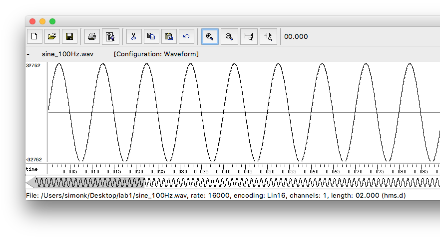
Load the example file sine_100Hz.wav from your sp/lab1 folder using the open command on wavesurfer’s file menu.
Wavesufer will ask you how you wish to display the file. For the moment just select waveform. If wavesurfer displays a pop-up error message when opening a file, you can ignore it.
You should see two version of the waveform on the screen. A big version at the top, which is the main display window, and a smaller version below it. This small version shows you which portion of the file is actually displayed in the top part of the window.
You can zoom in and out using the magnifying glass icons at the top of the window or by selecting a region by dragging the mouse over some of the waveform and selecting zoom to selection from the view menu (note the keyboard shortcuts on the menu for zooming).
To play the current selection, press the space-bar.
To see a spectrogram for a given file: Right click on the main waveform and select create pane and then select spectrogram. You can alter the detail displayed by right-clicking on the spectrogram and bringing up the spectrogram controls...
To see a spectrum, select a portion of the waveform and then right-click and select spectrum section...
For each of the non-speech waveforms:
- What are the differences between sine_100Hz.wav, sine_200Hz.wav and sine_300Hz.wav ?
- measure the time between 2 adjacent peaks in the waveform and calculate their fundamental frequency
- measure the amplitude
- Does the spectrum of a sine wave vary over time?
- What about the square and pulse waveforms? How do they differ from the sine waves?
- What is the relationship between the various waveforms? Are some more complex than others?
In the spectrum, the vertical axis is a logarithmic scale by default. So, we only need to focus on the peaks in the spectrum – this is where almost all the energy is. In the plot below, those peaks are at around 20dB. Don’t worry about the very low energy parts of the spectrum (between 60dB and 70dB in the plot below) – these are just artefacts of the analysis method.
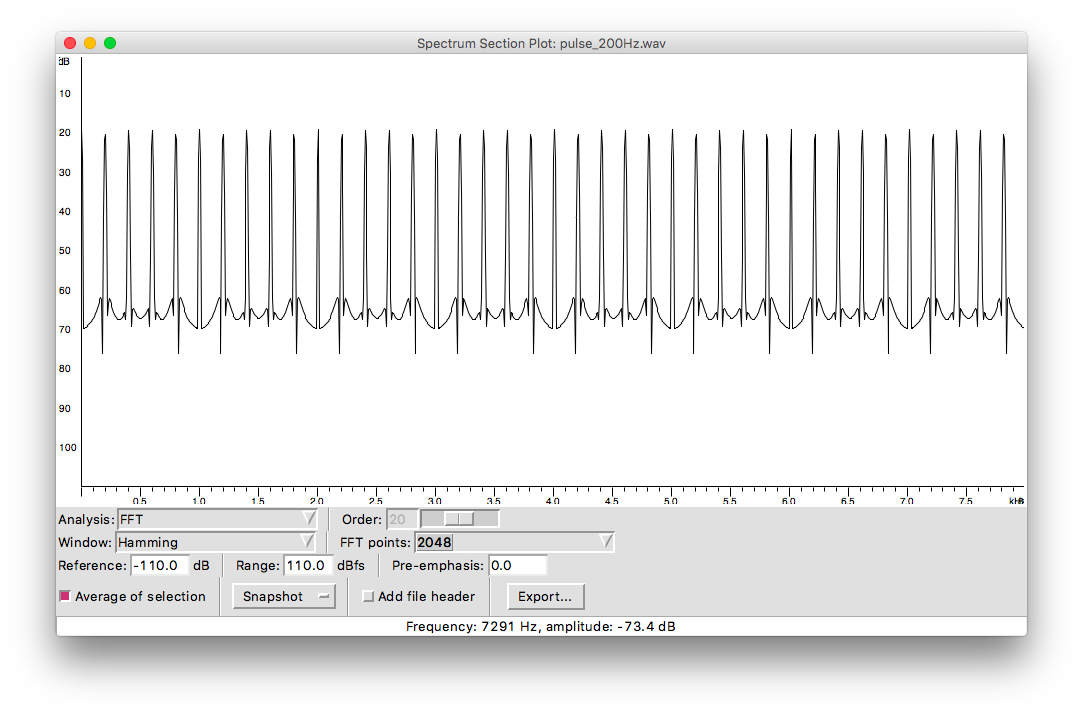
You can vary the frequency resolution of the spectrum by changing the FFT points setting: this controls how many samples from the waveform are analysed. Analysing more samples provides more frequency resolution.
For the speech waveform:
- Can you segment it into regions; how about using the spectrogram instead of the waveform?
- What patterns are emerging, and how does the waveform shape correspond to what you see on the spectrogram?
- Make spectra of different regions of the speech waveform. Use the snapshot button on the spectrum window to save a reference spectrum for comparison.
- For a single region (choose a vowel), try different analysis window lengths when computing the spectrum. What do you notice about the resolution of the resulting spectrum? Do the same thing in the spectrogram.
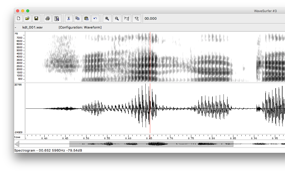
Some parts of speech signals have similar properties to the pulse train signal the you saw earlier. Here’s an example:
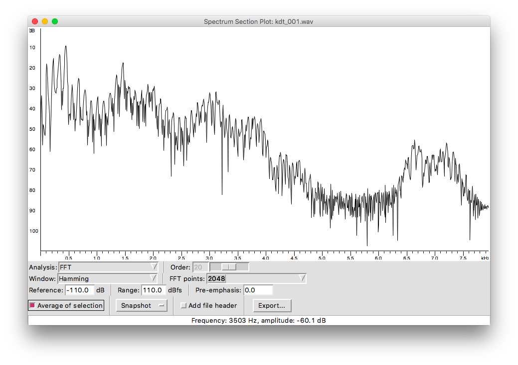
See how there is a similar “line structure”, at least in the lower frequencies. This tells us that there is something in common between speech and the simple pulse train. But there are differences of course. In the pulse train, all the lines (which are the harmonics) had the same height (which is the amplitude). In the speech signal, there is a more interesting shape (we call this the spectral envelope)
What does speech have in common with the pulse train? What causes speech to have a different spectral envelope to the pulse train?
There are some other parts of speech signals that don’t seem to have any harmonics. Here’s one example of this:
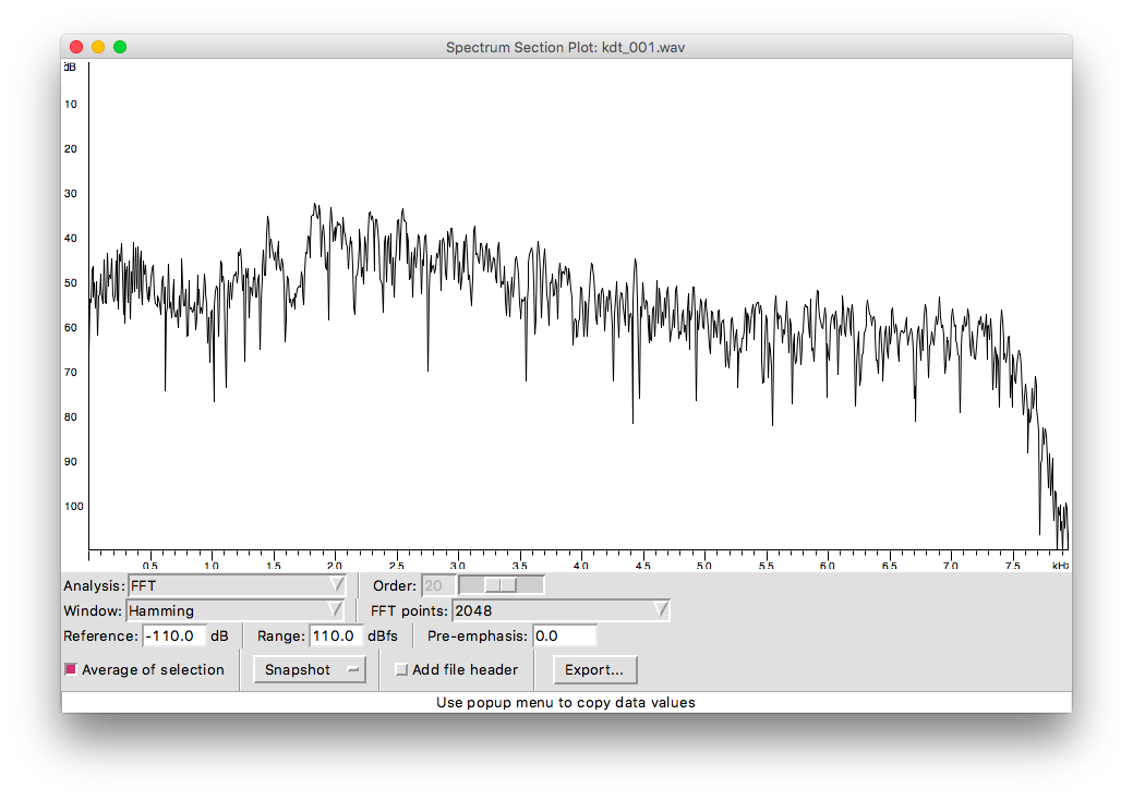
When does speech have no harmonics, and what does that tell us about how it was produced?