Module 9 – Speech Recognition – the Hidden Markov Model

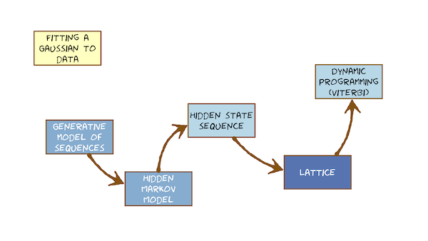
This video just has a plain transcript, not time-aligned to the videoTHIS IS AN UNCORRECTED AUTOMATIC TRANSCRIPT
A LIGHTLY-CORRECTED VERSION MAY BE MADE AVAILABLE IF TIME ALLOWS
we've been on a journey towards the hidden Markov model, and finally we've arrived.
We started by talking about pattern matching.
We did that with an algorithm called dynamic Time warping, in which we stored a template which is just a recorded example off.
Some speech would like to recognise, perhaps are isolated word called an exemplar on.
We matched that against some unknown speech that we would like to label when we measured distance between the store template on the unknown.
We then realised that this lacks any way of modelling the natural variability of speech.
The template is just a single store example.
It doesn't express how much we can vary from that example and still be within the same class.
So we decided to solve that by replacing the exemplar with a probabilistic model.
When we looked in our toolbox off probabilistic models and found the galaxy in is the only model that we can use.
It has the right mathematical properties, and it's very simple.
We're going to use the galaxy in the core of our probabilistic model, and that led us into a little bit of a detour to worry about the sort of features that we could model with a Gaussian.
We spent some time doing feature engineering to come up with features called MFC Sees that is suitable for modelling with diagonal co variance calc ins.
So now, armed with the knowledge of dynamic time warping on knowing its shortcomings and knowing that we've now got these excellent features called Mel Frequency Capture coefficients, we're ready to build a probabilistic generative model off sequences off M FCC vectors and that model good with the hidden Markoff model.
We're going to have to understand what's hidden about it.
What's Mark off about it, So to orient ourselves in our journey, this is what we know so far.
We talked about distances between patterns we saw.
There's an interesting problem there of aligning sequences of varying length.
We found a very nice algorithm for doing that called dynamic programming on the instance e ation of that algorithm dynamic time warping, and we saw that we could do a dynamic time warping.
We could perform the algorithm of dynamic programming on a data structure called a grid, and that's just a place to store partial distances.
We're not going to invent the hidden Markov model.
We'll understand what's hidden about it.
It's it's state sequence on that's connected to the alignment between templates on DH Unknown State sequence is a way of expressing the alignment.
And then we'll develop an algorithm for doing computations with hidden Markov model that deals with this problem of the hidden state sequence.
That data structure is going to be called a lattice, and it's very similar to the grid in dynamic time warping.
Think of it as a generalisation of the great, And so we're now going to perform dynamic programming on the different data structure on the lattice that will be doing dynamic programming for Hidden Markov models on the album gets a special name again.
It's called the Viterbi Algorithm.
That's the Connexion between dynamic time warping as we know it so far and hidden Markov models as we're about to learn them.
So we know that the single template in dynamic time warping doesn't capture variability.
Though many solutions proposed that before someone invented that Hmm.
For example, storing multiple templates to express variability that's a reasonable way to capture variability is a variety of natural exemplars.
The hmm is going to leverage that idea, too.
It's not going to store multiple examples, it's going to summarise their properties in statistics.
Essentially, that just boils down to the means and variances of Gazans.
So although there are ways of dealing with variability in down every time warping we're not going to cover them.
We're going to go straight into using statistical models, where, in some abstract feature space, let's draw a slice of capital features base forthe first of the seventh capital, coefficients of some sliced through this cultural feature space.
We're going to have multiple recorded examples off a particular class on rather than store.
Those were going to summarise them as a distribution, which has, I mean on DH, the standard deviation along each dimension or variance if you prefer.
So here's what we're going to cover in this module module eight.
You already know about the multi very galaxy in a generative model, a Multivariate Gaussian generates vectors.
We're going to start calling them observations because they emitted from this generative model.
We know that speech changes its properties over time, so we're going to need a sequence ofthe Galaxy ins to generate speech to need a mechanism to do that.
Sequencing on that amounts to dealing with duration.
We're going to come with a very simple mechanism for that which is a finite state network.
And so when we put these galaxy and generally models into the states of a finite state network, we got the head of Markov model.
We're going to see when the model generates data.
It could take many different states sequences to do that, and that's why we say the state sequence is hidden.
It's unknown to us, and we have to deal with that problem.
One way of doing that is to drive the data structure, which is the hidden Markov model replicated every time instant that's called the Lattice.
We're also going to see that we could perform dynamic programming directly on a data structure that is the hidden Markov model itself, and that's an implementation of difference.
Both of those are dynamic programming for the hidden Markov model.
On both of those ways of doing things, either the lattice well, this computation directly on Hidden Markov model itself are the Viterbi algorithm.
When we finish, all of that will finally remember that we don't yet have a way of estimating the parameters of the model from the data.
So everything here in module eight we're going to assume that someone's given us the model.
Some pre trained model.
We don't have the algorithm for training the model yet, so the very end will make a first step towards that will just remind ourselves how we contrarian a single gal.
Sian on some data might call that fitting the galaxy into the data or estimating the mean on variants of the galaxy.
And given some data, we'll see that that is easy.
But the hidden state sequence property of the hmm makes it a little harder to do that for hidden Markov model on a sequence of observations.
But that's coming in the next module.
So we know already that a single galaxy in a Multivariate Gaussian Khun generate feature vectors.
Are we going to call them observations? Let's just to remind ourselves that they are generated by a model.
Let's just make sure we fully understand that again.
I draw some part of our feature space.
I can't draw in 12 dimensional FCC space or higher, so I'm always going to draw just two of the dimensions any too.
It doesn't matter.
Two of the nfcc coefficients.
How does a Gaussian generate while the calcium is I mean, I mean is just a point in the space and we have a variance along each of the featured I mentions we're going to steam was no co variance.
And so variants of standard deviation in this direction, perhaps in this direction.
So one way of drawing that is to draw the contour line one standard deviation from the mean like that this model Khun generate data points.
What? I mean, it means we can randomly sample from the model on DH.
It will tend to generate samples near the mean on just how spread they are from the mean is governed by the perimeter variants.
So if I press the button on the model to randomly sample it generates a data point or one of the data point or another data point just occasionally a data point far from the mean.
More often than not, they're never mean so generous data points that have this Gaussian distribution.
That's the model being a generative model.
But we're not doing generation.
We're not doing synthesis of speech.
We're doing recognition of speech.
So what does it mean when we say there's a generative model.
Well, it says we are pretending.
We're assuming that the feature vectors extracted from speech that we observe coming into our speaks recognise er we're really generated by a Gaussian.
We just don't know which galaxy in on.
The job of the classifier is to determine which of the Garson's is the most probable galaxy into have generated a feature vector.
Of course, the feature vectors weren't generated by gas in their extracted from speech, and the speech for generated by the human vocal tract were making an assumption.
We're assuming that their distribution is galaxy in that we could model with a generative model as a gas in distribution.
So it's an assumption now, since these blue data points were extracted from natural speech on what we're trying to do is decide whether they were generated by this galaxy, and we don't really generate from the galaxy in we just take the gassings parameters.
We take one of these data points.
We compute the probability that this observation came from this calcium.
We just read that off the Gaussian curve as the probability density on we'll take.
That's proportional to the probability so the core operation we're going to do with our galaxy and generative model whilst doing speech recognition is to take a feature vector and compute the probability that it was emitted by a particularly calcium.
And that's what the garrison equation tells us.
It's the equation of the curve.
That's the equation that describes probability density in one dimension.
Got the Gaussian distribution along comes from Data Point, and we just read off the value of probability density.
It's that simple.
When we do that in multiple dimensions, with an assumption of No Cove Arians, we'll just do the one dimensional case separately.
For every dimension a multiply, all the probability density is together to get the probability off the observation vector, and that's an assumption of independence between the features in the vector.
So that mechanism off the multi variant calcium as a generative model, it's going to be right in the heart of our hmm that we're about to invent it solves the problem off the Euclidean distance measure being too naive.
How does it solve it? Because it learns the amount of variability in each dimension of the feature vector and captures that's part of the model the Euclidean distance measure only knows about distance from the mean it doesn't have a standard deviation parameter.
We cast our minds back to dynamic time warping, and just remember how that works.
This is the unknown, not the time running through the unknown.
This is a template that we've stored will assume that the first frame of each always aligned with each other because speech has been carefully end pointed.
There's no leading silence with a line.
This frame with this frame and then down any time warping just involves finding a path to hear.
That sums up local distances along the way, and those local distances are Euclidean.
Distance is here.
The galaxy is going to solve the problem off the local distance.
Let's take a local distance in this cell between this factor, this factor, and it's going to capture variability.
Storing a single frame of exemplar doesn't capture variability.
That's the main job of the galaxy in.
But there's another problem off templates.
It doesn't capture variability in duration, either.
There's a single example on arbitrarily chosen example of a recording of a digit say, Maybe this is a recording of me saying three.
The duration of that is arbitrary.
It doesn't model the variation in duration.
We might expect.
The template might also be a little bit redundant.
It might be that all of these frames sound very similar there.
The vowel at the end of the world.
Three.
We don't need to store three frames.
For that.
We could just store one or even better, because starve the meaning, the variance of those frames.
So we're going to get rid of the storey exemplar.
Are we going to get to choose the temporal resolution off the thing that's replacing it? The thing that's replacing it's going to be not an example, but a model.
And so my example are hard seven frames.
But maybe I don't need seven frames to capture the word three.
Maybe it's made off just three different parts.
Three different sounds.
So at the same time as getting with the exemplar, I'm going to gain control over the temporal resolution.
The granularity off my model on DH.
For now, let's choose three.
This is a design choice.
We're going to get to choose this number here, and we can choose it on any basis we like, But probably we should choose it to give the best accuracy of recognition by experimentation.
So where I used to have frames oven exemplar.
I'm now going to instead store the average on DH, the variance off those.
And I'm going to do that separately for each of the three parts.
So for this part here, I'm going to store a Multivariate Gaussian in the same dimensions, the feature space and it's going to store.
I mean, under variants on DH for the post of this module, not going to worry about where they come from.
I'm just going to assume that we will later devise some mechanism.
Some algorithm for training this model.
We're always going to see him for the rest of this module that the model has bean pre trained.
It was given to us.
So instead of storing an exemplar here, I'm going to store a calcium.
I'm going to draw one in one dimension because I can't draw in this many dimensions going to be a mean.
I understand the deviation, or we could still the variance for the middle part.
Going to store another one is going to be potentially different, mean on a different standard deviation and for the final one, the third one and yet another mean another standard deviation.
So where they used to be, a sequence off feature vectors For each of these three parts, there is now a statistical description of what that part of the word sounds like.
So this access is the model on the model is in three parts.
It models the beginning of the word, the middle of word and the end of the word, and we'll just leave it like that is a little abstract.
Certainly we're not claiming that these are going to be phoney names on DH.
We've already said that it doesn't have to be three.
It's a number of our choosing, and we'll worry about how to choose it another time.
So the model so far is a sequence off three housing distributions.
I've drawn them in one dimension, but in reality, of course, they're multi vary it on.
All we need now is to put them in some mechanism that makes sure we go through them in the correct order that we go from the beginning to the middle to the end bond the mechanism that also tells us how long to spend in each of those parts.
The duration of the unknown is going to be variable every time we do recognition.
That might be a different number, as we'll see when we developed a model the length of the observation sequence here, general going to be longer on the number of parts in the model.
And so we've got to decide whether this Gaussian generates just this frame or the first two, or maybe the first three.
And then when we how do we move up to the next gas into start generating the next frames on when we move up to the next gas ian, start generating the remaining frames? Sony's a mechanism to decide when to transition from the beginning of a word to the middle of a word from the middle of the world to the end of the world.
The simplest mechanism that I know to do that is a finite state network.
Let's draw finite state network.
We're going to build a transition between states on these transitions, say that we have to go from left to right through the model.
We don't go backwards.
Speech doesn't reverse on.
We now need a mechanism that says that you, Khun from each of these states generate more than one observation.
Remember, these are the observations, and that's just going to be a self transition on the state.
Inside the states are the multi very gas fumes that I had before with their means and variances.
So we started with a generative model off a single feature vector a Multivariate Gaussian on.
We've put it into a sequencing mechanism of finite state network that simply tells us in what order to use our various galaxy ins on DH.
We have some transitions between those states that controls that, and we have some self transitions on the state that allow us to emit more than one observation from the same Gaussian.
Those transitions are our model of duration.
We just invented the hidden Markov model.

This video just has a plain transcript, not time-aligned to the videoTHIS IS AN UNCORRECTED AUTOMATIC TRANSCRIPT
A LIGHTLY-CORRECTED VERSION MAY BE MADE AVAILABLE IF TIME ALLOWS
hidden Markov model comprises a set of states in each state is a Multivariate Gaussian on that gassing can emit observations.
Each time we arrived in a state of the model, we emit an observation, and then we must leave the state.
Now we must leave along one of a set of transitions that dictates what sequences of states are allowed.
The mother would you saw was a very simple model with a topology, a shape called left to right.
So the transitions the Ark's between the states govern that on because there are transitions from a state to itself, we can end up back in the same state on this, emit more than one observation from the same state.
That's a very simple model of duration.
So here's the mother we just invented.
This one's now got five emitting states.
I've drawn a one dimensional galaxy in the state just to show that there is a galaxy in there.
But of course there will be multi vary it.
So let's have this model emit or generate a sequence of observation vectors.
These are our observation factors.
For example, are MFC sees these lines indicate emission generation Two words for the same thing on this picture shows a five state hidden Markov model emitting a sequence of observations in a particular way.
The first emitting state emits the first observation in the sequence.
And then we go around the self transition and emit the second.
And then we go around the self transition again and admit the third.
And then we leave.
We arrived in the second emitting state, and then we generate the next observation.
In the sequence, we go around the self transition and in it, the next one.
We go around the self transition and emit the next one and then we leave.
And then we admit to the next observation sequence.
Every time we arrive in the state, we must emit an observation and then leave.
So this time we leave along the self transition and in it another one from that state.
And then we leave.
We met this one.
We leave back in the same state for one more time back in same set again, another observation.
And then we leave.
You make an observation, go around emitting observation, and we don't.
Hopefully it's already immediately obvious that there might have been another way of going through the model to generate this observation sequence.
What I just drew There was one particular state sequence for this particular state sequence.
We can compute the probability of this observation sequence, given the model, and it's just going to be the product of all the emission probabilities.
So off this calcium generating, the first observation multiplied by property of discussing generative next observation multiplied all the way through the sequence on DH.
We could also put some probabilities on the transitions.
So as we go around transition, there might be a probability on that.
That's right.
One is quite a high probability of going down this transition, so we'll multiply by all the transition probabilities.
Transition problems is leaving anyone state have to some upto one because there's a probability distribution over all the subsequent states.
The probability of this model emitting this observation, sequins and using this particular state sequence is just the product of all the emission probabilities on all the transition probabilities.
And it's that very simple product because the model assumes that the probability off emitting this observation sequence only depends on the state you omitted from, and that's all.
So the probability off this state emitting this observation and then emitting this observation and then emitting the next observation is just computed independently as the product of those three probabilities.
The model doesn't know.
It doesn't remember what it did in the previous time.
Step, that lack of memory that independence off.
One observation in the sequence from the next, given the hmm state is the Markoff assumption.
That's where Markoff, in the word hidden Markov model comes from.
This model has no memory.
Well, it's a very strong assumption on DH.
It might not be entirely true about this particular observation sequence, but that's the assumption the model makes.
No, this picture is the most common way of drawing a picture of a hidden Markov model.
It's the one you'll see in textbooks.
It's actually potentially really confusing.
That's a model, and that's an observation sequence.
Quite clearly, this is time in frames, for example, 10 milliseconds apart, that much is clear.
This is not time.
This particular model happens tohave a topology shape in other words, a set of allowable transitions that is left to right.
So we're clear going to move through the model in that order.
But this is a perfectly valid model.
This is a completely valid, hidden Markov model now.
It might not be particularly useful for doing speech recognition with, but it's a valid model.
And so any algorithms that we develop must work for this model as well.
As for this model.
This picture is potentially extremely confusing, because the model on the top on the sequence of observations of the bottom are not both along the same time access.
Only the observations have a time access.
The model is just a finite state model.
We could draw the model on its side, upside down, back to front with same model.
The layout on the page has no meaning to draw a picture that's much clearer.
The model is a model it always exists.
Exists now exist in the past, only exist in the future and exists every time.
Step off the observation sequence, first or picture that makes that completely explicit.
I'm going to draw a copy of the model, but every time step, this is time in frames, so we're stepping through that one frame at a time.
I was going to draw out a copy of the model good to duplicate it or unroll it over time.
We're just all the states.
That's the model at a time.
One that time, too.
Time three and so on.
I'll draw a copy of this model, but every time frame.
This is just a statement that the model always exists.
It's always there for this particular model.
This is the starting state.
And so the first observation in my observation sequence is always going to have to be emitted by that state because that's where we are at a time.
One and so that says we must be here.
And we can't be in any of these other states because we haven't time to go down the transitions to get there.
I'm going to also assume that we must finish in this state.
So I'm going to define that as the end state of the model.
When the model has generated observation Sequels.
It must always end up in that state and no other state.
And that means that that state must always generate the last observation.
The sequence.
That's a statement that we must be here and not here, and so we've got to get from here.
So here we've got to get through the model following the allowable transitions as we go through the observation sequence, Onda model generates observation secrets.
While we do that, this is starting to look quite like dynamic time warping.
That's deliberate.
So a generative model of sequences is the hidden Markov model, which is made off a finite state machine on those states contained gas Ian's and now we need to deal with the problem off this model.
And it's the same problem I had in dynamic time, warping that the alignment between the model on the observation sequence is not known to us.
Here's the potentially confusing version of the picture again that the model on the top we got the observation sequence along the bottom.
I showed the earlier one particular state sequence one particular way, going through the model and generating this observation sequence.
But there are many, many more ways of doing that, just like there are many, many possible alignments between a template and an unknown in dynamic time warping.
We can draw on alignment on this picture.
Let's just make one up.
And if I number thes states, that's just number them this way.
12 for five now I've drawn a state sequence that is 1111233344555 But you could go away on work out all the other state secrets is the possible.
You have to start with one, and they have to end with five.
But there are many, many permutations there.
Remember what we're doing when we're using a hidden Markov model to do pattern recognition.
We're assuming that one of our hidden Markov models that we've stored did generate this observation sequence.
Our only task is to work out which one could do it with the highest probability, which was the most likely model to have generated it.
It will be one of the models, but we don't know what state sequence that model used to generate this observation sequence.
And so we say that the state sequence of the hidden Markov model is hidden from us, and that's the definition of hidden in hidden Markov model.
It's that many possible state sequences could have been used to generate the observation sequence on We don't know which one.
It wass on the left is what I really want to compute.
I want to compute the probability of an observation sequence given a particular model.
I'm going to repeat that for all the models I've got on.
Pick the model that gives him the highest value and use that to label the observation sequence O on the right is what we've already seen.
How to compute.
We can compute the probability observation sequence on taking a particular state sequence.
Q.
So cute is a random variable, and it says state sequence, for example, Q might take the value 1112223 for five.
And if we know the state's sequence, we can compute the problem to the observation sequence in that state sequence.
To compute this joint probability here, how can we get TiVo, given the joint probability of P and O on cue, both conditioned on the model? Given this particular model, well, there's an easy way to do that.
We just some overall, the possible values of Q.
That's a simple rule of probability.
This operation is called marginalising or something away.
Q.
Now I just told you that there might be a lot of possible values of Q.
Q.
Is the state sequins on? The longer the model gets them along, the observation sequence gets the more values of cure possible.
It could be a very, very large number.
So this summation could be a very large summation.
It could be computation expensive to do this summation, but this is the correct thing to do for the hidden Markov model.
We really want to compute the probability of an observation sequence.
Given that model, we must sum over all possible state sequences the probability, the observation in that state sequence.
So we must summit away, marginalise it out because that computation is potentially very expensive.
We very often make an approximation to it and will say that approximately equal to finding the best cue, the best single value of Q.
So we just take the maximum overall possible vise of Q of this thing here toe pick one state sequence, the one that gives you the highest probability and assume that that's so much better than all the rest that that is a good enough approximation to the sub that turns out to be empirically a very reasonable thing to do.
This worked well in practise.
We could do the summation.
We could replace it with this maximisation operation on our speech, Recognise er will work just as well.
It will give justice lower word error rate.
How do you find the Q that maximises thiss probability.
We've got to search amongst all the values of Q.
But we don't want to enumerate them out, because then we might as well just do the summation.
We want a very efficient algorithm for exploring all the different values of Q.
The state sequence on DH minimising the amount of computation needed to find the best state sequence.
Well, that sounds awfully familiar.
Who defined the Hidden Markov model? And we've had it has this property state sequence.
That's the journey we need to take through the model to emit an observation sequence.
We don't know what state sequence our model took when it generates a particular observation sequence, I said.
The correct thing to do is to treat the state sequences a random variable to marginalise it away to some over it.
The summation could be very expensive, so we'll make an approximation.
We'll take a short cut and just say, Just find the most likely single state sequence.
Compute the probability of that state sequence generating observations on We'll take that as the probability that this model generated this observation sequence.
We need a data structure on which to do that computation that computation off, finding a single most likely state sequence whenever, say, state sequence, you could also hear alignment between the model and the data.
And then you could think that's just the same as dynamic time warping.
We're going to now create a data structure for doing that computation and is going to have to generalise to any shape of hidden Markov model any topology, any pattern off transitions of connexions between the states.
It mustn't be restricted to the case are very simple models that move from left to right.
Although the speech almost all our models will be like that.
We don't want an algorithm that's in the restricted case.
We wanted general algorithm.
We want to date a structure on which we could do that algorithm.
So that's what we're going to invent now.
So start again with dynamic time warping in dynamic time warping.
We had an algorithm called dynamic programming and to store the computations whilst doing the algorithm.
We needed a data structure and we made a date a structure called the grid.
That's the grid on each cell in the grid stores the partial path distance from the beginning to this point, that's the best so far.
We saw that the core computation in dynamic time warping was to find all the different ways of arriving in a cell on the grid and to only keep the best one.
So the court operation here walls a men over distances to take the minimum while minimum over distances and maximum over probabilities.
That's the same thing.
Just think of one's being that one over the other.
So men over distances and Max over probabilities are the same thing.
And so this suggests the sort of data structure that we might use for a hidden Markov model might look something like the grid.
The great is a bit too restrictive because it requires us to go left to right through this sequence, left right through this sequence.
That's fine for a template in an unknown.
We're going to replace this with a finite state network that could have any topology.
It might not necessarily go left to right, so the data structure we're going to use is called a lattice so on the right is a lattice for this hidden Markov model here with three emitting states.
I'm now going to start drawing my hidden Markov models in a way that matches the way that H t.
K implements them.
It's going to turn out to be extremely convenient later, when we need to join models to other models going to add non emitting started end states.
I'm going to start numbering.
That is number one.
The first emitting state was number two and so on.
Through the model, we're going to switch now to H T K style models.
This is an implementation of detail, but is going to make something later much easier.
So I must start in my non emitting state in the lattice, and I must end in by final non emitting state.
So they're the definitions away.
We must start and end in dynamic time, will think we had a rule, a rule that we had to invent about how you can move through the grid.
We said that the rule was this one, or the rules are available.
If you go and read the old literature or rather all textbooks, you'll find that there are other possible patterns of moving through grid, but this is the one we stuck with.
The simplest.
The counterpart of that in the hidden Markov model is that the model topology connexions on DH.
The lack of connexions between certain pairs of states tells us how we can move through the lattice.
So this model says that from the non emitting start state, you must always go to the first emitting state.
That's that one there.
When you arrive there, you must emit the first observation that's done.
And then time advances.
One step.
We must take a transition at every time step and then who arrive in the state and generating observation.
The topology of this model says that you could stay in the same state when time moves forward.
Or you could move to the next state when time moves forward so you could stay in the same state.
Well, you could move to the next state, so it's impossible to get to this state to admit the first observation.
Auto this one.
So these will never be visited in the lattice, and then we generate this observation.
Now we could generate it from this state or this state.
So we do both, and we store both computations separately, those air to partial paths through the lattice.
We don't know which one is best yet.
They're in different states.
We store them both.
We have to parallel path.
Civilian competition in parallel were exploring all possible alignments between model on observation sequence.
And this says that there's two different paths alive at the moment and we can't get there.
And we've generated this observation sequence first one on the second one, and then we move forward in time again.
The topology of the model says that from this state you can stay in the same state or move forward.
But if you were still here, then you could move forward and we'll stay in the same state and so on.
So he just used the topology of the model to fill up the lattice.
Now we have to end up here, so these paths that leaves the model too early and no good.
That's equivalent to coming out of the end of the model.
But not having generated all the observation sequences, we haven't accounted for them all, so that's not a valid path through the model these ones were already said.
You can't even get there and we can see that this one is a dead end.
There's no way to get to the end in time, and so is this one.
And so the lattice is this picture here and this lattices thie exact counterpart to the grid and dynamic time morphing, and we would do computation on it in exactly the same way.

This video just has a plain transcript, not time-aligned to the videoTHIS IS AN UNCORRECTED AUTOMATIC TRANSCRIPT
A LIGHTLY-CORRECTED VERSION MAY BE MADE AVAILABLE IF TIME ALLOWS
So I've seen that there's a transition of ideas from dynamic time warping, where the data structure wass a simple grid to this new data structure for the hidden Markov model called the Lattice, where the allowable transitions between the states in the lattice are dictated by the topology of the model, not by some simple external rule.
So the lattice is a general data structure that would work for any shape, any topology off.
Hmm.
When on that lattice on that data structure, we can perform the algorithm off dynamic programming.
When we apply that to the hidden Markov model, it gets the special name off the Viterbi algorithm.
So we done with dynamic time warping.
We learned it because it's a nice way to understand dynamic programming.
We've had this transition now to the hidden Markov model in a good way.
To think about the hidden Markov model is a generalisation off dynamic time warping with templates.
The template.
The store exemplar was a bit arbitrary.
It was just one recording off someone saying This digit, for example, Andi didn't capture variability either, acoustically around the average way of saying it or indeed, in terms of duration, is just one particular way of saying it.
So we've generalised replaced that with a model.
In general, the model have fewer states than there were frames.
In the template is a generalisation.
Each of the state's contains a Multivariate Gaussian that expresses a statistical description off what that part of the word sounds like.
So, for example, it replaces thes three exemplar frames with their means and variants on the model has a transition structure transitions between the states that does the job off, going through the model in the right order.
So for most models in speech that will be left to right on DH off, how long to spend in each part of the model? And that's a model of duration, the very simple model of duration.
But it is a model of duration, so it's very important that Allah Grant developed for the hidden Markov model doesn't rest on this left to right topology, even if it is the most common, I might occasionally want to use them all that has this transition, for example, maybe I'll have a model ofthe silence that could just go round and round, generating as much silences.
I need beginnings and ends of utterances that might put that transition in the model.
For that purpose, the lattice still works.
Most restore the lattice for this particular topology that has this transition going from the third emitting state back to the first one, or in h d K.
Language from the fourth state to the second state because the non emitting one gets numbered one.
So for this model, let's draw the lattice.
Well, the lastest apology just dictated by the model.
So from this state, we could go here or here.
There should be arrows and all of these from the state.
Same thing from this state we can narrow.
Go to the non emitting final state or self transition.
Oh, go back to hear.
Go here.
Well, leave.
It would be leaving too early.
All go back to the start.
Yeah.
Ah, back to the start.
Yeah, the back to the ah, yeah, Back to there.
This lattice is a little bit more complicated, but it's still just a set off states joined by transitions on any algorithm that we can perform on the simple artist we can perform on this one on.
What we're going to see now is that we can do the computations on that lattice.
That's a perfectly reasonable way to do it on this data structure or we confined.
Actually, an alternative implementation, which uses the hmm itself is the data structure.
So actually, there are two ways at least to implement the Viterbi algorithm for Asia.
Mum's one is to make the lattice on to perform dynamic programming on the lattice.
You start here, you go to the first emitting state, you admit on observation.
Then you either go here or here, and you admit the next observation in sequence.
Now, each state gets to emit that observation in general, imitate with a different probability and update the probability of the partial path so that the two partial paths alive at this point, and they'll compete later when they meet.
But for now, we must maintain both of them.
So we're doing a parallel search and then we'll just propagate forward through the model like that.
There's a one way of doing it.
But there's another way of doing it directly on the hmm structure.
So I'm going to make a connexion for you now between the way of doing it on the lattice to the left.
That would be how most textbooks describe the algorithm andan algorithm, which is going to use the hmm itself on the right as the data structure.
It's not going to make the lattice never going to draw this lattice out.
He's going to use the H members, the data structure on It's gonna be equivalent.
And that algorithm is called token passing.
Along comes a sequence of observations, and we're going to emit them in sequence.
So is the first one on the left will have made the transition to this state.
I will admit it and compute the probability of doing that on the right.
Would have put a token here, will have sent the token down an ark.
It will arrive here.
We use that galaxy in to admit that observation will update the tokens probability with that probability and then comes in the next observation in sequence.
We'll go forward here and compute that go forward here and in it it again from a different state.
But two different state sequences possible.
Now this is the state sequence.
22 This is the state sequence two three amusing actually K numbering the counterpart over here would be that one.
Copy.
The token goes around self transition and ends up back here.
Another copy, the token Because the next state and end up here, This one emits the observation.
And so does this one on the update.
Their probabilities.
We have two tokens alive in the model at once.
This token, the same as this point in the lattice.
This token is the same as this point in the lattice.
And then we just turn the handle on the algorithm, repeating those steps over and over again.
So things I mean something in the middle of the algorithm.
At some point, we're generating this observation on DH.
Imagine we were going to generate it from here from this emitting state.
Two paths will have arrived from previous time.
Step will have done the max operation to keep only the most probable.
And then we'll generate this observation from the Gaussian off this state on update that probability they're the counterpart of that will be over on this side.
Were arriving in this state.
One token will have come from this direction.
One token will be self transitioning token.
That was already in that state of the previous time step, We'll do the max to keep just the most likely those two tokens on DH.
Discard the other one, and then we limit this observation and update the tokens.
Probability hopefully can see that The thing of the laughter, the thing on the right of doing the same computation on the left.
We need a data structure which is a lattice on the size of the lattice is going to be governed by the length of the observation sequence on the number of states in the model.
Now, that doesn't seem very big here because our eventual observation sequence this has got five observations, and our model only has three emitting states.
So our lattice only has 15 states in it, but in general, are models might be much, much bigger than that.
Observation sequences might be considerably longer tens or hundreds of frames long, and so this lattice could get quite large and use a positive memory.
So the implementation on the right could use a lot less memory because it only uses thie.
Hmm.
Itself is the data structure.
So the size of its data structure is just the size of the hmm.
How does the algorithm on the right get to you? So little memory? Well, essentially, it's just computing this and then this and then that could be discarded.
And then this that could be discarded.
And then this could be discarded, and then this.
Then that could be discarded.
So token passing is actually just a very particular form of search on the lattice.
It's called time synchronous.
It computes in strict order off time.
On the only needs as much memory is the hmm hmm exists each time.
So this one, it's token.
Passing one on the left is the search on the lattice.
And we could imagine in this lattice that we might not want to strictly explore it in this order.
That's only one way of doing it.
We already saw in dynamic time warping there's other ways of doing it.
We could explore it in more interesting orders.
For example, that will be not time synchronous would have moved through time before we'd finished going through all the model states.
But for the person of this course, we're only really bothered about time synchronous search on Soto comm Passing is a perfectly good way to understand the Viterbi algorithm for H.
M.
M's.
So you know the hmm.
Now it's a finite state network, and inside each state, is there Gaussian acting as a generative model.
It can generate a single observation, and then we must leave the state.
Either go around a self transition or to another state.
It doesn't matter.
The model topology tells us what's allowed on.
Every time we arrive in the state, we use its calcium to emit the next observation in sequence.
We've only seen that for a single hidden Markov model.
I have been saying all the time that the way that we do classification is by having one hidden Markov model for each of the classes that we want to recognise on DH will compute the probability of each of them generating observation sequence and pick the highest.
What's coming next is actually a way off connecting all the models together to make a single hidden Markov model not off necessarily isolated words, but of a sentence made of words.
So connected speech.
And that extension, because we've used finite state models, will turn out to be really quite easy.
All we need is something that tells us how to join models of words together to make martyrs of sentences.
And then we can generalise further and say, Let's model sub word units, for example.
Let's model phone aims.
And then we need something else that tells us how to join Foa names together to make words.
So the thing that tells us how to join words together to make sentences is called a language model.
And as long as it's finite state, as long as we restrict ourselves to models of language that are finite state, there'll be no difficulty in.
Combining with the hmm is to make a single, large, finite state model.
So this part is going to be easy connected speech.
The elephant in the Room The thing we haven't talked about throughout is how to actually learn the model from data.
Now.
You might think it would have been sensible to do that at the beginning and then to use the model to do recognition.
Because, of course, that's what we do.
Want to build a system that's the hard way to learn it much easier to understand what the models doing when it's emitting an observation sequence, its computing, the probability join doing recognition almost have understood all of that.
We can use that knowledge to understand the hardest part of the course overall, and that's how to learn the modern from data we call that training Computational E is going to be straight forward.
It's going to involve very much the sort of computations we just saw there on the lattice.
That's an attractive property.
They hit a mark off model that its computational e straightforward to train to learn from data.
But conceptually, you're going to find it perhaps the most challenging part of the course, which is why we left it toe last till we're comfortable about H.
M.
M's on about how to do recognition with them.
You got a good memory.
From the beginning of this module, you'll see that there's something missing from this picture.
We haven't done it yet on that wass fitting galaxy into data.
Well, we've mentioned that several times so far, so let's just first, we have a quick recap and see how that helps us in learning a hidden Markov model from data.
That's the equation for the galaxy.
In when have you seen this equation? You zoom in on this part and then zoom in on this part and see first a Euclidean distance.
And then the Euclidean distance scaled bye variants, scaled Euclidean distance, and then the rest equation just makes it into a nice bell shaped curve with an area of one.
This course isn't about proofs, so we're not going to do a proof for how to estimate the parameters of the gas.
And we're going to stay them and then say that they look quite reasonable.
So what are the parameters mean on variants? Mu on Sigma Squared is a unit, very a Gaussian.
But that's all we need because we're assuming no co variance everywhere.
How do you estimate the mean on the variance of a galaxy in from some data? Well, first of all, you need some data, so let me write down some data points.
It was some notation next one, thanks to next, really aren't necessarily in any sequence.
There just data points.
There's no idea of ordering to the data points that training Allison.
It has no model of sequences, some big bag of data points.
Let's have an off hm n data points on these data.
Points are labelled data.
They're labelled as having come from this calcium, the label with class that this garrison is modelling.
The requirement for labelled data to estimate the model parameters is normal in machine learning.
We say that the machine learning this then supervised and that's the only sort of machine learning we're covering in this course where the data are labelled with a class that were modelling.
I'm going to state without proof that the best possible estimate of the mean of the galaxy in is the mean of the data.
I'm going to write down that my best estimate.
That's what little hat means.
My best estimate off the mean of the galaxy in is the empirical mean the mean, found through experimentation found from data.
And that's just going to be out of all the data points and divide by how many there were.
This estimate of the mean is the one that makes this data the most probably can be given the calcium.
So we can say that this estimate is a maximum likelihood estimate off the mean concede that intuitively, by setting you to be the mean of all the axis will make on average, this term of smallest possible, and that will make the probability as large as possible.
Morgan State without proof that the best estimate off the variance is going to be the variance of the data, that the variance of the data is the average squared.
Distance off the data from the means or the average squared deviation.
And we can see that intuitively, because the variance is scaling the squared distance between data and mean.
So I'm going to write that my empirical estimate ofthe variants Syrians hat is going to be the squared distance between data and mean summed up over all the data on divided by harmony data points worth the average squared distance from the mean.
I'm going to state those without proof as being the most reasonable estimates.
And they are.
We could prove that these are the estimates that make this data of the highest possible probability maximum likelihood.
Given this calcium, that's fine.
There's a lovely, simple, easy formula.
They work in one step, take the data, average it you've got the mean with that estimated mean take the data again.
Look at the average squared distance from the mean on DH.
That's your variants, but that required this data to be known to come from this one gal Siem.
Unfortunately, that's not the case for the Hidden Markov model.
Imagine I am fitting this hidden Markov model to this one observation sequence I've labelled This sequence is having come from the model, but I I'm not able to label which frame in the sequence comes from which state of the model? Because the state sequences hidden.
I don't know that.
And I am trying to estimate the mean on variants of the galaxy in here based on the data, and I don't know exactly how the model aligns with the data.
That's a problem to be solved in the next module.
And that's an algorithm for training the hmm, Given the data, we've seen that if we could find on alignment between the states and the observations, we could just apply those simple formula for estimating the meaning, the variants.
But the fact that the state secret is hidden makes finding this alignment nontrivial that's to be solved in the next module