Foundation concepts you need for this module
Before starting this module, you may want to revise the optional foundation material on Probability again. In particular, you need to understand the properties of Gaussian probability density functions, and why modelling covariance requires so many parameters. This provides the motivation for the step in feature engineering where we try to eliminate (or substantially reduce) covariance.
If you are unsure what the logarithm is, then you should go through all the “Logarithms” videos in this foundation material on mathematics.
Module content
This module introduces the concept of feature engineering, in which the features are manipulated to make them more suitable for whichever type of machine learning we have decided to use.
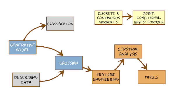
Here’s what you’re going to learn in this module:
Lecture Slides
Slides for Thursday lecture (google)
Total video to watch in this section: 44 minutes (divided into 4 parts for easier viewing)
Here are the slides for these videos.
Assumptions & references made in these videos
The opening slide in the video “Intro to Generative Models” says “Module 7” – this is now Module 8.
The video “Intro to Generative Models” assumes familiarity with discrete and continuous (random) variables, and Bayes rule. The foundation material on probability will be enough for you to understand this video, so go over that first if you need to. We will then consolidate these topics in the lecture for this module.
The last slide in the video “From MFCCs, towards a generative model using HMMs” states that HMMs are in Module 8: that should now read Module 9. It states that estimating the parameters of an HMM is in Module 9: that should now read Module 10.
This video just has a plain transcript, not time-aligned to the videoTHIS IS AN AUTOMATIC TRANSCRIPT WITH LIGHT CORRECTIONS TO THE TECHNICAL TERMS This module has two parts.In the first part, we're going to start building the hidden Markov model, but only get as far as deciding to use Gaussian Probability Density functions as the heart of the modeland that will make us pause for thought and think about the features that we need to use with Gaussian Probability Density functions.So in this first part, going to introduce a rather challenging concept.And that's the idea of a generative model and we'll choose the Gaussian as our generative model for the features we have speech recognition.The main conclusion from that part will be that we don't want to model covariancethat is, we're going to have a multivarite Gaussian - that's a Gaussian in a feature space that's multi-imensional: feature vectors extracted from each frame of speech.We would like to assume that there's no covariance between any pair of elements in the feature vectorfor the features that we've seen so far (filterbank features) that's not going to be true.So those features are not going to be directly suitable for modelling with a Gaussian that has no covarianceparametersWe call such a Gaussian "Diagonal Covariance" because only the diagonal entries of its covariance matrix have non-zero values.We'll conclude that we want diagonal covariance Gaussians.We'll realise that filterbank features are not suitable for that.And we need to do what's called 'feature engineering' to those features: some further steps of processing to remove that covariancethat will result in the final set of features that we're going to use in this course, which are called Mel Frequency Cepstral Coefficients (MFCCs).To get to them, we'll need to understand what the cepstrum is.Let's orient ourselves in the course as a whole.We're on a journey towards HMMs.We've talked about pattern matching.We've seen that already in the form of dynamic time warpingthere was no probability therewe were comparing a template (an exemplar) with an unknown and measuring distance.The distance measure was a Euclidean distance for one feature factor in the exemplar compared to one feature vector in the unknown.The Euclidean distance is really what's at the core of the Gaussian probability density functionour conclusion from doing simple pattern matching was that it fails to capture the variability of speech: the natural variability around the meanA single exemplar is like having just the mean.But we want also the variability around that.That's why we're moving away from exemplars to probabilistic models.So to bridge between pattern matching and probabilistic generative modelling, we're going to have to think again about features because there's going to be an interaction between the choice of features and choice of model.In particular, we're going to choose a model that makes assumptions about the features.And then we need to do things to the features to make those assumptions as true as possible.We've already talked enough about probability and about the Gaussian probability density function in last week's tutorials.We've also covered why we don't want to model covariance.We also looked at human hearing, and we decided to take a little bit of inspiration from how the cochlea operates.The core reason we don't want to model covariance is that it massively increases the number of parameters in the Gaussian, and that would require a lot more training data to get good estimates of all those parametersWe're not going to explicitly model human hearing.We're going to use it as a kind of inspiration for some of the things we're doing in feature extraction.So without repeating too much material from last week, let's have a very quick recap of some concepts that we're going to need.We're modelling features such as the output of a filter in the filterbank.That's a continuously-valued thing.So we're going to need to deal with continuous variables, but also we're going to need to deal with discrete variables.At some point, we're going to decide speech is a sequence of wordswords are discrete: we can count the number of typesmaybe we're going to decompose the word into a sequence of phonemesthat's also a countable thing: a discrete thing.We're going to need to deal with both discrete and continuous variables, and they are going to be random variables.They're going to take a distribution over a set of possible values or over a range of possible values.An example of a discreet variable, then, will be the word, and in the assignment that will be one of the 10 possible values.An example of a continuous variable will be the output from one of the filters in the filterbank, or indeed, the vector of all the outputs stacked together.That's just a vector space, and that is also a continuous variable in a multi-dimensional spacewe need different types of probability distribution to represent them.But apart from that, everything else that we've learned about probability theory and in particular this idea of joint distributions, conditional distributions, and the all-important Bayes' formula - the theorem that tells us how to connect all of these things - applies to both discrete and continuous variables.It's true for all of them.In fact, eventually we're going to write down Bayes' formula with a mixture of discrete and continuous variables in it: words and acoustic features.But that won't be a problem because there's nothing in all of what we learned about Bayes that tells us it only works for one of the other.It works for both discrete and continuous variablesSo I'm not going to go over that material again.I'm going to assume that we know that.So let's proceed.We can use probability distributions to describe data, as a kind of a summary of the datawhen we do that, we're making an assumption about how those data are distributed.For example, if we describe data using a Gaussian distribution we assume that they have a Normal distributionwe might even make some stronger assumptions: that they have no covariance.But before choosing the Gaussian, let's stay a little abstract for a while.We're not going to choose any particular model.We're going to introduce a concept: a difficult concept.This will be difficult to understand the first time you encounter it.It's a different way of thinking about what we do when we have a model.What is a model?What is a model for?What can it do?We're going to actually build the simplest possible form of model.So a generative model is actually a simple as it gets, because a generative model can only do one thing: it can generate examples from its own classso there's a difficult concept to learn.But it's necessary because it allows us to build the simplest form of model: the generative model.So here's the conceptual leap.Here are three models of three different classes A, B and C.We keeping this abstract!I'm not saying anything about what form of model we're usingThese are black boxesand the only thing that a model can do (for example, Model A here) is emit observations.Let's make it do that.The observations here are balls, and they have one feature: the colour.So that just emitted a blue ball.Well, that's all this model can do.We can randomly emit observations: we can generate from the model.So let's generate.There's another one generating observations.The observations are data pointsand so on, and we keep generating.So this is a random generator, and it generates from its distribution.So inside Model A is a distribution over all the different colours of balls that are possible.And it randomly chooses from that, according to that distribution, and emits an observation.So keeping things abstract and not making any statements about what form the model has (it's not got any probability distribution) what are we going to say about model A?Well, we could imagine it essentially contains lots and lots of data from Class A - like thatand we might have other models, too, for other classes.And we could imagine for now that they just contain a lot of examples of their classes ready to be generated - ready to be emittedWhat will B and Model Cand you can see that it seems likely that Model A is going to emit a different distribution of the values (of colours) to Model Band Model B is going to emit a different distribution to Model C.So let's see what we could do with something like that.these are generative models: all they can do his emit observationsalready, and keeping things very abstracte, without saying anything about what type of model we're using, let's see already that this simple set of three models (A, B and C - one for each of the classes) can do classification.Even though all the models can do is emit observations.They don't make decisions, but we can use them to make decisions: to classify.So let's he how a set of generative models can together be used to classify new samples (test samples)So incomes a data point.There it is: a ball, and its feature is 'green'I would like to answer the question "Which of these models is most likely to have generated it?"If I can find the most likely model, I will label this data point with the class of that modelwe'll keep the models abstract by pretending that they just contain big bags of ballsSo that's what the models look like inside.So we try and generate from the model, and we make the model generate this observation.One way of thinking about that, if you want to think in a frequentist way (a 'counting' way) is to emit a batch of observations from each model and count how many of them are green - that's the frequentist view.The Bayesian view is just to say, "What's the fraction / What's the probability of emissions of observations from our model that are green?"Now we can look at Model A it's pretty obvious that it's never going to emit a green ball.So the probability of this green ball having being emitted from Model A is a probability of zero.I'l write it with one decimal place for precision.Look at Model B.It's also clear, just by looking, that Model B never emits green balls either.the probability of that emitting a green is 0.0.Now let's look at Model C.You can see that model C emits blue balls and yellow balls and green balls - let's say - with approximately equal proportions.So there's about a 0.3 probability of model C emitting a green ball.Clearly, this is the largest probability of the three so we'll classify this as being of class CNotice that each model could compute only its own probability.It didn't need to know anything about the other models to do thateach model made no decisions.It merely placed a probability on this observed green ball.We then made the decision by comparing the probabilities.So the classifier is the comparison of the probabilities of these models emitting this observation.That's what makes these model simple: that they don't need to know about each other.They're all quite separated, and in particular when we learn these models from data we'll be able to learn them from just data labelled with their class.They won't need to see counter-examples.They won't need to see examples from other classes, and that's the simplicity of the generative model.Other models are available: models that might be called 'discriminative models' that know about where the boundaries between - for example, Class A and Class B - are and can draw that decision boundary and directly make the decision as to whether an observation falls on the Aa side of that line or the B side of that line: of the classification boundary.These models do not do that.We have to form a classifier by comparing the probabilities.Let's classify another observation.So along comes an observation and our job is to label it as being most likely Class A or Class B or Class C.We just do the same operation again.We ask Model A: "Model A, what is the probability that you generate a red ball?"We can see just visually from model A maybe emits red balls about two thirds of the time.So Model A says "The probability of me emitting a red ball is about 0.6."Ask Model B: "Model B, what's the probability that you emitted a red ball?"Well, we look and model B emits red balls and yellow balls and blue balls they are in about equal proportion.It says "I can emit red balls and I can do it about a third of the time.""Model C, what's the probability that you emitted the red ball?"Well, it never emits a red ball: 0.0.How do we make the classification decision?We compare these three probabilities.We pick the largest and we label this test sample with the class of the highest probability model, which is an A.So this is labelled as AWe have done classification.So you get the idea, along comes a sample.You ask each of the models in turn: "What's the probability that this is a sample from you / from your model / from your internal distribution (whatever that might be)?"We compute those three probabilities and pick the highest and label the test sample with that class.So, as simple as generative models are, we can do classification simply by comparing probabilities.
This video just has a plain transcript, not time-aligned to the videoTHIS IS AN AUTOMATIC TRANSCRIPT WITH LIGHT CORRECTIONS TO THE TECHNICAL TERMS Let's move on from discrete things, from coloured balls to continuous values because that's what our features for speech recognition arethey are extracted from frames of speech, and so far where we've got with that is filterbank features: a vector of numbers.Each number is the energy in a filter (in a band of frequencies) for that frame of speech.So we need a model of continuous valuesthe model we're going to choose is the Gaussian, so I'm going to assume you know about Gaussian from last week's tutorial.But let's just have a very quick reminder.Let's do this in two dimensions.So I just take two of the filters in the filterbank and draw that two dimensional space.Perhaps I'll pick the third filter and the fourth filter in the filterbank.each of the points I'm going to draw is the pair of filterbank energies: a little feature vector.So each point is a little two dimensional feature vector containing the energy in the third filter and the energy in the fourth filterso: lots of data pointsI would like to describe the distribution of this data with a Gaussian, and it's going to be a multivariate Gaussianthe mean is going to be a vector of two dimensions.and its covariance matrix is going to be a 2x2 matrix.I'm going to have here a full covariance matrix, which means I could draw a Gaussian that is this shape on the data.We've made the assumption here that the data are distributed Normally and so that this parametric probability density function is a good representation of this data.So I can use the Gaussian to describe data.But how would we use the Gaussian as a generative model?Let's do that.But let's just do it in one dimension to make things a bit easier to draw.I've got my three models againBy some means (yet to be determined) I've learned these models - they've come from somewherethese models are now GaussianSo this is really what the models look like.Model A is this GaussianIt has a particular mean and a particular standard deviation.along comes an observation.So these are univariate Gaussian: our feature vectors are one dimensional feature vectorsSo along comes a 1-dimensional feature vector (it's just a number)the question is "Which of these models is most likely to have generated that number?"the is number 2.1remembers that the Gaussian can't computer probability - that would involve integrating the area between two values.So, for 2.1 all we can say is, "What's the probability density at 2.1?"So off we go2.1 this value ... 2.1 this value ... 2.1 this value.Compare those three.Clearly, this one is the highest.And so we'll say this is an A.That's how we'd use these three Gaussians as generative models.We'd ask each of them in turn, "Can you generate the value 2.1?"For a Gaussian, the answer's always "Yes!", because all values have non-zero probability (density)(.So of course, we can generate a 2.1.What's the probability density at 2.1?We just read that of the curve because it's a parametric distributionand compare those three probability densitiesso we do classification with the Gaussian.Let's just draw the three models on top of each other to make it even clearer.What's the probability of 2.1 being an A or a B or a C?Well, just go to 2.1 and you've got this probability density, this probability density, and this probability densityClearly A is the highest and it's an ABy drawing the models on top of each other, we can actually see the implicit decision boundaries between the classes.It's obvious that up to here A is always the highest value.So this whole region here will always be labelled Athis region in the middle here, the B probability density function is higher than the other two so everything in that region will be labelled as a Band for the remainder, going this way, everything will be labelled CSo thes three Gaussian generative models - whilst not knowing anything about each other - when we lay them on top of each other, we can see that they do form decision boundaries.Thiese three Gaussian form a classifier, and it has boundaries here and hereand divides feature space (which is this whole range of the variable) into three parts and labels one with A, one as B, one with Cbut those boundaries and never stored.We never need to know thosethey arise simply by comparing the probabilities (in fact, the probability densities) of any observation valuethat works in two dimensions.pick some pair of filters Let's pick the the 4th one and the 5th oneLet's have two classes now, so let's have class green.It's got the mean here.That's the mean of class green.It's got some standard deviation in the two feature directions, so let's draw a Gaussian there.This has got full covarianceLet's have class PurpleLet's have it's mean and it's standard deviation in all directions.Maybe that looks like this: it's much tighterow there's going to be - as we move around this feature space, trying all these different points - some will be more likely to be green and some will be more likely to be purplethere is an implicit decision boundary between the two classes, maybe the decision boundary is going to look something like this, perhapseverything here has got a higher probability (higher probability density) of coming from the purple distribution and everything here has got a higher probability density of coming from the green distribution.This classification boundary between the two classes is never drawn out explicitly.If it was that will be called a 'discriminative' model.That's not what we're doingThis is a generative model and we have to find that boundary simply by comparing the probability densities of the two models.And if there are more models, we will get more complicated decision boundaries.So that completes the first part of the class.We want to use Gaussians because they have nice mathematical properties.We want to use generative models because they're the simplest sort of model.We know there isn't anything simpler.We're going to use Gaussians as the generative model of the feature vectors - feature vectors coming from frames of analysis from our speech waveformwe've seen that generative models can be used to classifyultimately, the problem of speech recognition is one of classification.It's one of saying: "Which words were said, out of all the possible words? Which ones were most likely?"So we're going to do that through generative modelling.Now our Gaussians are going to be multivariate: they're going to be in some high dimensional space feature space - it's going to have tens of dimensions.At the moment it's the number of filters in the filterbank.And if we were to model covariance, that would have a very large dimension covartiance matrix[The number of entries in the covraiance matrix would] be proportional to the square of the dimension of the feature vectorThat's bad.So we're going to now do something to the features so that we don't need to model covariance.We going to do feature engineering.
This video just has a plain transcript, not time-aligned to the videoTHIS IS AN AUTOMATIC TRANSCRIPT WITH LIGHT CORRECTIONS TO THE TECHNICAL TERMS So on with the remainder of the class, which is all about feature engineeringwe'll start with the magnitude spectrum on the filterbank features that we've seen before in the last module.Quick recap.We extract frames from a speech waveform.This is in the time domain.We extract short term analysis frames[and use a tapered window] to avoid discontinuities at the edgeswe apply the discrete Fourier transform and we get the magnitude spectrum.This is written on a logarithmic scale.So this is the log magnitude spectrum, and from that we extract filterbank features.filterbank features are found from a single frame of speech in the magnitude spectrum domain.We divide it into bands spaced on the mel scale.Sum up the energy in each band and write that into element of the feature vectortypically we use triangular-shaped filters and space their centres and their widths on the mel scale so they get further and further apart and wider and wider as we go up frequency in Hzand the energy in each of those into the energysum this one is written into the first element of the feature vector: a multi-dimensional feature vector.Now let's make it really clear that the features in this feature vector will exhibit a lot of covariance: they're highly correlated with each otherThat will become very obvious when we look at this animation.So remember that each band of frequencies is going into the elements of this feature vector extracted with these triangular filters.So I will to play the animation.Just look at energy in adjacent frequency bands.Clearly the energy in this band and the energy in this band are going up and down togethersee that when this one goes up, this one tends to go up.When this one goes down, this one tends to go down.They're highly correlated.They covary because they're adjacent and the spectral envelope is a smooth thing and so these features are highly correlated.If we wanted to model this feature vector with the Multivariate Gaussian, it will be important to have a full covariance matrix to capture that.So the filterbank energies themselves are perfectly good features unless we want to model with a diagonal covariance Gaussian, which is what we've decided to do.So we're going to do some feature engineering to get around that problemwe're going to build up to some features called Mel Frequency Ceptral Coefficients - or MFCCs as they are usually calledthey take inspiration from a number of different directionsOne strong way of motivating them is to actually go back and think about speech production again and to remember what we learned a little while ago about convolution.Knowing what we know about convolution, we're going to derive a form of analysis called Cepstral analysis.Cepstral is an anagram of spectral: it's a transform of spectral.Here's a recap that convolution in the time domain (convolution of waveforms) is equivalent to addition in the log magnitude spectrum domain.So just put aside the idea of the filterbank for a moment.Let's go right back to the time domain and start again.This is our idealised source.This is the impulse response of the vocal tract filterif we convolve those (that's what star means), we'll get our speech signal in the time domainthat's equivalent to transforming each of those into the spectral domain and plotting on a log scaleAnd then we see that log magnitude spectra add together.So this becomes addition in the log magnitude spectrum domainconvolution is a complicated operationWe might imagine (perfectly reasonably) that convolution is very hardin other words, given that, to go backwards and decompose it into source and filter from the time domain is hard.But we could imagine that undoing an addition is rather easier.And that's exactly what we're about to do.How do we get from the time domain to the frequency domain?We use the Fourier transform.The Fourier transform is just a series expansion.So to get from this time domain signal to this frequency domain signal we did a transform that's a series expansionthat series expansion had the effect of turning this axis from time in units of seconds to this axis in frequency, which has units of what? Hz.But Hz = 1 / s.So this series expansion has the effect of changing the axis to be 1 over the original axis.So we start with something in the time domain and get something in the "1 / time" domain = frequency domain.So that's a picture of speech production.But we don't get to see that when we doing speech recognition!All we get is a speech signal which we can compute the log magnitude spectrum of.What would I like to get for doing automatic speech recognition?Well, I've said that fundamental frequency is not of interest.I would like the vocal tract frequency response.That's the most useful feature for doing speech recognition.But what I start with is this.So can I undo the summation?That's how speech is produced.But we don't have access to that.We would like to do this.I would like to start from.We can easily compute with the Fourier transform from analysis frame of speech.We would like to decompose that into the sum of two parts: filter plus sourcethen for speech recognition, we'll just discard the source.How might you solve this equation, given only the thing on the left?One obvious option is to use a source-filter model.We could use a filter that's defined by its difference equation.We could solve for the coefficients of that difference equation and that will give us this part.And then we could just subtract that from the original signal and whatever is left must be this part here, which we might then call the 'remainder' or more formally call it the 'residual' and we'll assume that was the source.That will be an explicit way of decomposing into source and filter: we would get both the source on the filter.Actually, we don't care about the source for speech recognition.We just want the filter, so we could do something a bit simpler.Fitting an explicit source-filter model involves making very strong assumptions about the form of a filter.For example, a resonant filter (all pole) and that different equation has a very particular form, with particular coefficients.We might not want to make such a strong assumptionsolving for that difference equation (solving for the coefficients, given a frame of speech waveform) can be error proneand it's actually not something we're covering this coursewe want to solve this apparently difficult-to-solve equation where we know the thing on the leftwe want to turn it into a sum of the two things on the right.These two things have quite different looking properties with respect to this axis here, which is frequency.This one's quite slowly varying, smooth and slowly varying.It's a slow function of frequency with respect to the frequency axis.This one here quite rapidly moving.It changes rapidly with respect to frequency.So we would like to decompose this into this slowly varying part and that rapidly varying partI mean slowly and rapidly varying with respect to this axis, the frequency axis.I can't directly do that into these two parts, but I can write something more general down like this.I can say that a log magnitude spectrum of an analysis frame of speech equals something plus something plus something plus something and so on...where we start off with very slowly-varying parts and then slightly quicker-varying all the way up to eventually very rapidly-varying parts.Does that look familiar? I hope so!It's a series expansion, not unlike Fourier analysis.So it's a transform.We're going to transform the log magnitude spectrum into a summation of basis functions weighted by coefficients.Well, we could use the same basis functions as Fourier analysis.In other words, sinusoids with magnitude and phase.Or any other suitable series of basis functions.The only important thing is that the basis functions have to be orthogonalso they have to be a series of orthogonal functions that don't correlate with each other.Go and revise the series expansion video if you need to remember what that is.In this particular case, for a series expansion of the log magnitude spectrum, the most popular choice of basis functions is actually a series of cosines.where we just need the magnitude of each.There's no phase there, just exactly cosinesthat suits the particular properties of the log magnitude spectrum.So we're going to write down this.This part here equals a sum of some constant function times some coefficient (a weight).Plus some amount of this function: that's the lowest frequency cosine we can fit in there, time some weightPlus some amount of the next one, plus some amount of the next one, and so on... for as long as we likehere's a suitable [series of] orthogonal basis functions.That's a cosine series.It starts with this one, which is just the offset (the 'zero frequency' component, if you like)and then works its way up through the seriesAnd so we'll be characterising the log magnitude spectrum by these coefficients.This is a cosine transform lots and lots of textbooks give you really, really useless and unhelpful analogy to try and understand what's happening here.They'll say the following to say:Let's pretend this is time and then do the Fourier transformWell, we don't need to do that!A serious expansion is a serious expansion.There's nothing here that requires this label on this axis to be frequency, time, or anything else.You don't need to pretend that's the time axis.You don't need to pretend this is a Fourier transform.This is just a series expansion.You got some complicated function and you're expressing it as the sum of simple functions weighted by coefficients.It's those coefficients that characterise this particular function that we're expanding now.How does this help us solve what we wanted to solve?We just write this thing (this magnitude spectrum) as just the sum of two parts:A slowly-varying part with respect to frequency, that we'll say is the filter.And a rapidly-varying part we'll say is the sourcebecause here we've got some long series of parts.Well, we'll just work our way up through the series and at some point say that's as rapidly-varying as we ever see the filter (with respect to frequency) and we'll stop and draw a line.And everything after that we'll say is not the filter.So we'll just count up through this series and at some point we'll stop and we'll say: the slow ones are the filter and the rapid ones are the source.So all we've got to do in fact now, is decide where to draw the lineand there's a very common choice of value there, and that's to keep the first 12 basis functions, counting this one as number one.This is a special one.It's just the energy and we count it as zero.So that's the first basis function, the second, the third, when we go up to the 12thAgain, in other descriptions of cesptral analysis, particularly of the form used to extract MFCC, you might see choices other than the cosine basis functionsyou could use a Fourier series, for examplethat's a detail that's not important.The important thing is - conceptually - this is a series expansion into a series of orthogonal basis functionsexactly what functions you expand into is less important.We won't get into an argument about that!We'll just say cosine series.What is the output off that series expansion going to look like?Well, just like any other series expansion, such as the Fourier transform, we'll plot those coefficients on an axis.This is frequency in Hz.Frequency is the same as 1 / time.Remember that a series expansion gives you a new axis that is "1 / the previous axis".So 1 / (1 / time) is ... time !So actually, we gonna have something that got a time axis, a time scale.This is going to be the size of the coefficient of each of the basis functions.So we're going to go for 1,2,3,4,5,6,7,8,9,10,11,12 basis functions.But at that point will say: these guys belong to the filter and then everything else to the right we're actually going to discard because it belongs to the source.But let's see what it might look like.Well, we just have some values.This thing is gonna be hard to interpret.It's going to be the coefficients off the cosine series.But what will we find if we kept going well past 12?At some point there would be a coefficient at some high time where we get some spike again.Let's think about what that means on the magnitude spectrum.So this is the cosine series expansion.These lower coefficients here...Now, this is is time.But because this is a transformed from frequency 'onwards', we don't typically label it with time.We label it with an anagram of frequency and people use the word quefrency.Don't ask me why!Its units are seconds.So this low quefrency coefficient is the slowly moving part.One of these, perhapsHere is some faster-moving part - up here some faster-moving part.Perhaps this oneAnd eventually this one will be that one that moves at this ratethis is a cosine function that happens to just 'snap onto' the harmonics.It would just match the harmonics.So this one here is going to be the fundamental period (T0).Because this matches the harmonics - F0For our purposes, we're going to stop here.I'm going to throw away all of these as being the fine detail and retain the first 12: 1 to 12.So this truncation is what separates source and filter.specifically it just retains the filter and discards the source.Truncation of a series expansion is actually a very well-principled way to smooth a function.So essentially we just smooth the function on the left to remove the fine detail (the harmonics) and retain the detail up to some certain scaleand our scale is up to 12 coefficients.
This video just has a plain transcript, not time-aligned to the videoTHIS IS AN AUTOMATIC TRANSCRIPT WITH LIGHT CORRECTIONS TO THE TECHNICAL TERMS Now what we just saw there was the true cepstrum, which we got from the original log magnitude spectrumthat's going to inspire one of the processing steps that's coming now in the feature extraction pipeline for Mel Frequency Cepstral Coefficients.So let's get back on track with that.We've got the frequency domain: the magnitude spectrum.We've applied a filterbank to that, primarily to warp the scale to the mel scale.But we can also conveniently choose filter bandwidths that smooth away much of the evidence of F0We will take the log of the output of those filters.So when we implement this, normally what we have here is the linear magnitude spectrum, apply the triangular filters and then take the log of their outputsWe could plot those against frequency and draw something that's essentially the spectral envelope of speechwe then take inspiration from the cepstral transform.And there is a series expansion in that.We'll use cosine basis functions, and that's called cesptral analysisthat will give us the cepstrumthen we decide how many coefficients would like to retain, so we'll truncate that series typically at coefficient number 12and that will give us these wonderful coefficients called Mel Frequency Cepstral Coefficients.In other descriptions of MFCCs, you might see things other than the log here.Some other compressive function, such as the cube root.That's a detail that's not conceptually important.What's important is that it's compressive.The log is the most well-motivated because it comes from the true cepstrum, which we got from the log magnitude spectrum.It's the thing that turns multiplication into addition.This truncation here serves several purposes.It could be that our filter bank didn't entirely smooth away all the evidence of F0 and so truncation will discard any remaining detail in their outputs.So we'll get a very smooth spectral envelope by truncating the series to remove any remaining evidence of the source, just in case the filterbank didn't do it completely.That's number one.The second thing it does that we'll explain in a momentwe alluded to is that by expanding into a series of orthogonal basis functions, we find a set of coefficients that don't exhibit much covariance with each other.We removed covariance through the series expansion.Third, and just as interesting, we've got a place where we can control how many features we get.12 is the most common choice, but you could vary that.We get the 12 most important features, the ones that (capture) the detail in the spectral envelope up to a certain fineness of detail.It is a well-motivated way of controlling the dimensionality of our feature vector.So did we remove covariance?We could answer that question theoretically, which we'll try and do now.We could also answer that question empirically (= by experiment): we could do experiments where we use Gaussians (multivariate Gaussians) with diagonal covariance when we use filterbank features and compare how good that system is with MFCC.In general we'll find the MFCCs are betterThe theoretical argument is that we expand it into a series of orthogonal basis functions, which have no correlation with each other.They're independent, these are uncorrelate with each other.And that's the theoretical reason why a series expansion gives you a set of coefficients which don't have covariance - or at least have a lot less covariance than the original filterbank coefficients.So finally, we've done cepstral analysis and we've got MFCCs.MFCCs are what you're using in the assignment for the digit recogniserYou're using 12 MFCCs plus one other feature.The other feature we use is just the energy of the frame, and it's very similar to the zeroth cepstral coefficient (C0) but is just computed from the raw frame energySo you've actually got 13 features: energy plus 12 MFCCs.But when you go and look in the configurations for the assignment, or you go look at your trained models, you'll find that you don't have 13.You've actually got 39!It's part of the assignment to figure out how we got from 13 to 39-dimensional feature vectors.And now it's obvious why we don't want to model covariance in 39-dimensional feature space.We'd have 39 by 39 dimensional covariance matrices.We'd have to estimate all of those covariances from data.So coming next:we've got the Gaussian - that's going to do all of the workwe've seen that the Gaussian can be seen as a generative modelbut a single Gaussian can just generate a single data point at a time.But speech is not that.Speech is a sequence of observations: a sequence of feature vectors.So we need a Multivariate Gaussian that can generate one observation, one feature vector for one frame of speech.We need to put those Gaussians into a model that generates a sequence of observations.And that's going to be a Hidden Markov model.And that's coming up next.That's the model for speech recognition in this course.We've then got to think: Well, what are we going to model with each hidden Markov model?We're going to generate a sequence of feature vectors for a whole word.That's what we're going to do in the assignment, because we've only got 10 words, so we can have just 10 models and we can have lots of examples of each of them to train those models on.We'll see eventually, that doesn't generalise well to very large vocabularies.So we're going to model sub-word units, and you might be able to already have a pretty good guess what a suitable sub-word unit might be.We also need to think about how we're going to make a generative model that could generate a sequence of observations (sequence of feature vectors) that's not just a word, but a sequence of words: a sentence.We got to do connected speech.Now it sounds like all of this stuff could be really, really hard.But it'll turn out that by making the hidden Markov model simply be a finite state model, this is easy because everything will be a finite state model.So the core ideas coming next:in module 8 that's the hidden Markov model and we'll get that model In just one remaining module we can cover everything we need to make a full connected speech recognition system by modelling sequences of words where the words are made of sub-word unitsThen we finish with actually the hardest part, which is how to estimate the parameters of the HMM.We've already thought about how we might do that for an individual Gaussian.I give you 74 data points, and I tell you they were all emitted from this particular class (= they were labelled with that class).You could easily fit a Gaussian to those 74 data points.For example, the mean will be the sum of the data points divided by 74.you could compute the variance as well.The problem with estimating the paramters of the HMM is that we won't know frame by frame, which Gaussian each frame is assigned toso we can't directly do that.We'll need to align the model and the dataso we need an algorithm for alignment.So estimating the parameters of the HMM is the hardest part of the course, so we leave it for last!However, we will see a way of aligning the model and the data much sooner than thatmWhen we want to do recognition with an HMM we will also have to decide how to allocate frames in the observation sequence to states in the HMM, so we can compute the probability of each observation coming from a particular state.That's an alignment problem between a model and the sequence of observations, and it's exactly the same problem as Dynamic Time Warping: alignment between two sequences.We can solve it with exactly the same algorithm: dynamic programmingwe'll call that the Viterbi algorithm: that's dynamic programming as used with a hidden Markov model.So that's where we're going.
Reading
Jurafsky & Martin – Section 9.3 – Feature Extraction: MFCCs
Mel-frequency Cepstral Co-efficients are a widely-used feature with HMM acoustic models. They are a classic example of feature engineering: manipulating the extracted features to suit the properties and limitations of the statistical model.
Wayland (Phonetics) – Chapter 9 – Hearing
Introduces basic concepts in human hearing - it may be useful to read the bits on decibels/loudness and the Mel and Bark scales.
Holmes & Holmes – Chapter 10 – Front-end analysis for ASR
Covers filterbank, MFCC features. The material on linear prediction is out of scope.
Taylor – Section 12.3 – The cepstrum
By using the logarithm to convert a multiplication into a sum, the cepstrum separates the source and filter components of speech.
In this module’s lab, you continue working on your ASR assignment.
This week you should aim to get your speaker independent digit recognition pipeline set up. This means writing scripts so that you can:
- Train your digit recogniser on speech data from multiple speakers in the course dataset
- Apply the digit recogniser to test set data from multiple speakers in the dataset.
- Make sure you can handle the case where the training set speakers and test set speakers are completely different people.
- Collate and evaluate the results of the digit recogniser in terms of Word Error Rate
Once you’ve got your speaker independent pipeline going, you should think about what experiments you want to focus on for the report write up. This means identifying some hypotheses and explaining why you think they will (or won’t) hold in specific experimental settings. You should support your arguments with sources from the literature (i.e., readings from the course and beyond).
Discuss potential hypotheses and experimental designs in with Simon and the tutors in the lab.
Private
- You do not have permission to view this forum.
If you read very recent papers on speech recognition, you’ll find that MFCCs are not as widely used as in the past. Instead, filterbank features are quite common. This is because the type of machine learning being used has changed from HMMs (with Gaussian probability density functions) to Neural Networks.
Nevertheless, the concept of feature engineering is still important in many areas of Machine Learning. Even the most powerful statistical models will not perform very well using unsuitable features.
What you should know
- What are generative models?
- Gaussian distributions:
- What shape is a Gaussian distribution?
- How do we describe a multivariate Gaussian in terms of means and variances
- How could this be used to tell us, for example, the probability that a specific feature vector is from a specific category?
- Cepstral analysis, filterbanks, MFCCs
- Non-linear speech perception: semitones, mel scale (from module 7)
- What do we want MFCCs to capture about each frame of speech?
- What are the steps used in generating MFCCs?
- What step makes these ”mel” frequency cepstral coefficients
- What step makes these features ”cepstral” coefficients?
- Why do we generally prefer to use MFCCs to Mel filterbank features in HMM based ASR?
- Why do we use MFCCs rather than the full magnitude or power spectrum in ASR?
- Why do ASR models often we use 39 features per frame (e.g., the configuration in Assignment 2)? What are these features?
- Why don’t we want our features to covary?
Key Terms
- generative model
- probability distribution
- Gaussian distribution
- mean
- variance, covariance
- standard deviation
- multivariate
- probability density function
- feature vector
- sampling
- cepstral analysis
- cepstrum
- filterbank
- mel-scale
- mel-frequency cepstral coefficients
- non-linear
- log scale
- spectral envelope
- Discrete Cosine Transform
- Inverse Discrete Fourier Transform
- magnitude spectrum
- power spectrum
- delta features
- acceleration (aka delta-delta) features