Make sure you’ve read everything in the Intermission module before proceeding.
Foundation concepts you need for this module
Revise the foundation material on mathematics from “Variables and indexes” up to “Functions”, and the recommended reading “Vectors and their uses” before watching the videos.
Module content
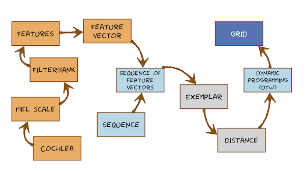
This is the start of the Automatic Speech Recognition material. In this module, we will make a preliminary attempt to extract salient features from speech signals, then use pattern matching to compare an unlabelled sample of speech to several stored samples with known labels (“exemplars”).
Start with this very simple post, which defines the problem as one of extracting a feature vector (here with just 2 dimensions) and then doing pattern matching by measuring distance in feature space to exemplars:

But that won’t handle anything other than stationary speech sounds. We need a way to deal with words and sequences of words. The problem is non-trivial because it involves sequences of variable length. This is recurring theme in Speech Processing, and in Natural Language Processing more generally.
Now work through the videos and readings which introduces a simple approach to pattern matching for variable length sequences: Dynamic Time Warping.
Here’s what you’re going to learn in this module:
Lecture Slides
Thursday lecture slides (google) [updated: 7 Nov 2023]
Total video to watch in this section: 52 minutes (divided into 5 parts for easier viewing)
Here are the slides for these videos.
Assumptions & references made in these videos
“You already know that the waveform is not the right representation for pattern recognition” arises from material in the early modules of the course where, for example, we found that only the magnitude spectrum is required to distinguish speech sounds, whereas phase can be discarded.
“You have a reasonable idea of this concept of a feature vector” simply means that you already know why we need short-term analysis for speech signals (because their properties change over time) and that each analysis frame can be characterised by a set features, such as its magnitude spectrum. The videos in this modules build on this, and develop a better feature vector than the magnitude spectrum.
“In the previous videos, we suggested that linear time warping would be one possible solution.” There is no previous video now, so linear time warping will be mentioned in the lecture as a precursor to Dynamic Time Warping.
This video just has a plain transcript, not time-aligned to the videoTHIS IS AN AUTOMATIC TRANSCRIPT WITH LIGHT CORRECTIONS TO THE TECHNICAL TERMS This is the start off the speech recognition part of the course, and we're on a journey towards a model called the Hidden Markov model (HMM).We're gonna start with something much simpler than a model, something called pattern matchingThat's in this module.We'll then move on to thinking about the features that we extract from speech a bit more deeply.We will do some feature engineering and then finally will get to the hidden Markov model, which is a probabilistic generative model.Along the way, we're going to learn an algorithm called Dynamic Programming, and we're going to see that now in the form of Dynamic Time Warping.We'll see that when we move from pattern matching to a probabilistic model, we might have specific requirements for the features that we extract from speech.Some interaction between the model we use and the features that we choose.That's why we need to do feature engineering.Then we'll see Dynamic Programming again for the hidden Markov model in the form of the Viterbi algorithm.You already know that the waveform is not the right representation for pattern recognition.For example, it includes phase information, which we know isn't particularly useful for discriminating, for example, one phone from another.You have a reasonable idea of this concept of a feature vector, but we're going to develop that a little bit more in this video.We're going to throw away the waveform and replace it with a sequence of feature vectors.We're going to use the sequence of feature vectors for pattern matching, using a very simple method with whole word templates.But even this very, very simple and outdated method that we're going to talk about now already has to tackle the fundamental problem of dealing with sequences of different lengths.So you know, the way form is not a good representation because it combines source and filter, and it includes phase.We only want the filter, so we want something like the spectral envelope.We know that speech waveforms change over time and that we can use short-term analysis to deal with that on.We're going to extract a feature vector from each frame in a short term analysis of the speech wave formand to deal with this problem of sequences of different lengths, we're going to need an algorithmthe core of the algorithm is going to be about finding an alignment between two sequences.In the previous videos, we suggested that linear time warping would be one possible solution.Clearly, that's too naive.Speech doesn't behave like that.And so now we're going to develop the real algorithm, which is going to be a dynamic or non-linear time warping to align two sequences of differing lengths.So here's what we're going to learn.It divides into two parts.In the first part, we're going to extract features from frames of speech, and the destination of that first part is a sequence of feature vectors to replace the waveform, and that will be our representation of speech for doing pattern matching.In the second part, we'll take that sequence of feature vectors, and we'll match one sequence that we know the label for against another sequence that we're trying to put a label on.In other words, we're trying to do speech recognition.We'll find the distance between those two sequences of feature vectors.Let's start on the first part.In the beginning of this course, when we talked about signal processing and how speech was produced, we took some inspiration from speech production, and that led us to a source filter model, which we could use to explain speech signals and could be the basis for speech synthesis and all sorts of other things.That's still relevant.But also relevant would be some understanding of speech perception.So let's start with that, because we're going to take some inspiration from human speech perception to do feature extraction for automatic speech recognition.The cochlea is part of our hearing system.on this diagram, it's this part herethe cochlea acts like a bank off filters that respond to different bands of frequencies in this incoming audio.Of course, sounds coming isn't always speech, but we're only interested in speech hereso sound comes into the ear and it ends up in the cochlea.In our bodies, the cochlear is coiled into a spiral.But I is just to save space because we need to leave more room in ourhead for our brain!And so to understand that, we don't need to worry about it being a spiral.We can just draw it out as a straight structure like thisso sound comes into the ear is a sound wave, and it propagates down the cochlea on different places along the cochlea (this is place) respond to different frequencies in the incoming sound wavethey're effectively little resonating filters, each of them responding to a narrow band of frequenciesin some parts in the cochlea, those little resonating filters respond to high frequenciesOn the other end of the cochlea, they respond to low frequenciesso we can understand the cochlea, which is the device in our bodies that converts sound pressure waves into nerve signals to be sent off for interpretation by the brain, as a bank of filtersthe cochlea spreads frequency along its length: along placeOne of the most important features off this bank of filters in the cochela is that it's not spaced linearly on a Hertz scaleit's spaced quite non linearly.There's lots of mathematical functions that are used to approximate that non-linearity, the most common one in speech technology is called the mel scale.the male scale looks like thisas we linearly increase in Hertz, the mel scale is compressive.It curves this way.So, for example, the difference in Hertz here at these high frequencies is a relatively small difference in melbut down here, the same difference in Hertz is a much larger difference in mels.It is this compressive nature of this curve that's important.What that means is that human hearing is less sensitive to frequency differences up here in the high frequency range than in the low frequency rangewe're going to use that when we extract features from speech signals for speech recognition.We're going to extract more (= denser) features in this sort of frequency range, which happens also to be where all the information in speech isand fewer (= coarser) features up in the higher frequency range.So the cochlea is like a bank of filters, and they're spaced non-linearly in Hertz or linearly on some perceptual scale, such as the mel scale.We can use that along with our knowledge of the special envelope, to start extracting some useful features for automatic speech recognition.So let's see how a mel-scaled filter bank could be used to extract the spectral envelope from a speech signal.So here, when I say auditory system, I really just mean the peripheral part, the cochela: the bit that's converting sound waves into nerve impulses.We're not talking about any processing in the brain.Let's remember what a band pass filter is.It's something that has a lower frequency limit and upper frequency limit, and it extracts those frequencies from the input signal.It's easiest to draw in the frequency domain, where it rejects everything outside of its band.It accepts everything inside its band.That will be an idealised, perfect rectangular bandpass filter drawn in the frequency domain.The cochlea is like a set off such filters: a bank of filtersand they are spaced along a mel scale so they get further and further apart in Hertz at higher frequencies and their widths also get wider.So a simplified idea of what the cop theatres will be that there are banned past philtres like that.That's one of them, and then another one a little widerand then another one. Why do still and so on? I've just simplified the cochlear as only having four bands.Of course, it's got many more from that but we can see that the centre frequencies of these filters get further and further apart as we go upentire frequencies.and the width of these filters also get wider bandwidth.these are bandpass filters: they pass through a band of frequencies.Now these idealised rectangular bandpass filters aren't actually possible physically: the cochlea isn't like that.the cochela has a set of overlapping filters that have a more realistic shapeA slightly better approximation than a bank of rectangular filters will be a bank of triangle filters that overlap.So we might have filters that look like this: getting wider and wider and further and further apart.And the spacing here is on a mel scale.Again, I've just drawn four filters; we're going to use more than that to simulate what the cochlea does.So we've got a simplified model off the cochlea as a sequence of triangular filters: a bank of triangular filters.We're going to use that now to extract features from speech way forms
This video just has a plain transcript, not time-aligned to the videoTHIS IS AN AUTOMATIC TRANSCRIPT WITH LIGHT CORRECTIONS TO THE TECHNICAL TERMS So what do we mean by a feature?Well, one possible set of features for speech recognition would be the raw waveform samples themselves, but have already dismissed that as a representation that's not particularly useful.It includes phase and other things that we're not interested inAn alternative will be what we're seeing here, which is to discard phase and just look at the magnitude spectrum that's already better than the waveform because it's invariant to phase.Remember what we're seeing on this picture.This is the output of the Discrete Fourier Transform.There are bins, here, up to the Nyquist frequencyThat set off numbers could be a set of features for doing automatic speech recognition: the raw DFT features, but just the magnitude and not the phases.But we also know that this includes information that we're not interested in (in general) for doing speech recognition.We can see here that we can resolve all the harmonics of F0.In general, F0 is not a useful feature for speech recognition.What we would like would be something that's this envelope.So, and even more useful feature than a DFT bin would be the output of one of this bank of filters.So I've just drawn the filters.It rejects everything, then it passes its band with some response shape: here it's triangular.What is the output of this filter? If we put the speech signal through this filter, it would pass through all of these frequencies and reject everything else.What we're interested in is summing all of the energy in that band, summarising that as a single number for a particular analysis frame.It is the amount of energy in this frequency range and in that analysis frame.That's what we mean by the output of a filter.So each filter's output will be a useful feature for doing automatic speech recognition - even more useful than the DFT bins themselves.So we've got a bank of filters and each filter, for each analysis frame. summarises the amount of energy in its pass band and writes it out as a numberwhat we're going to now you're going to just store them into a vector.So here's a speech signal: it's in the time domainit's going to always be easier to think about everything in the frequency domain.So let's draw the magnitude spectrum.What's this? this is the magnitude spectrum for some analysis frame, so we've taken some section of speech signal, cut it out, we've probably applied a tapered window, and we've taken the DFT to get the magnitude spectrum.So that's frequency.We're going to extract from this magnitude spectrum a set of features.The features are going to be the amount of energy falling inside each of the pass bands off a bank of overlapping triangular filtersof some number of filters that we have to choose - but it's going to be something like 20 to 30 typicallywe're going to store each of those in a vector.The first one is going to produce some output.We'll store that in the first element of the vector, and then the next filter will summarise its energy into some output and we store it in the second element of the vector, and so on...Each vector stores the features for a single analysis frame: this analysis frame here.Now, speech changes its properties over time, and so we analyse it with a sequence of such analysis frames.So let's just talk a little more generally about this idea of sequences, because it's going to be the core problem we have to solve eventuallySequences are everywhere in language.A waveform is a sequence of samples.We can analyse that sequence of samples with a sequence of overlapping analysis framesThere is some correspondence between a frame and the samples that fall inside it.Back in speech synthesis, we could think about sentence being a sequence of words, a spoken word being a sequence of phones or a written word being a sequence of letters.Now we've gone from a waveform being a sequence of samples to being a sequence of overlapping analysis framesand each frame giving rise to a feature vector that's extracted from it.So a waveform has become a sequence of feature vectors.Now, what do all these sequences have in common?Well, they're all of variable length.There'se some alignment between sequences at one level on sequences at another.For example, phones aligned with words.But it's not trivial because the number of phones per word is variable.Or we might also want to align sequences of the same type.If we're building a spelling correction system, we might need to align two letter sequences: the sequence of letters somebody typed and the sequences of letters of all the words in our dictionary and compute something called the Minimum Edit Distance (or the Levenshtein Distance) to find the word that's closest to what they typed and correct it.We might have the output of a speech recognition system, which gets some words right and some words wrong.We'd like to compute its accuracy, or its word error rate (WER)That's something we'll need to do later in the course.And that will involve aligning two word sequences, which are potentially of different lengths and have a nontrivial alignment.What we're going to do here and now is going to align to speech signals represented by sequences of feature vectors.We're going to measure how similar they are.We're going to use that to do pattern matching and therefore to label unlabeled sequences with the label of the closest stored pattern that we already have.In spoken language processing, most of the time, the alignments between these sequences are monotonic.That is, as we advance through, for example, a sequence of words, we also advance through the sequence of phones that correspond to that sequence of words in a left-to-right fashion.We don't backtrack; there's no reordering.But the alignment isn't linear.We don't just move proportionally through the two sequences.It's nonlinear; it's dynamic.For example, the number of phones in the word varies word by word, and this dynamic alignment is also going to be true when we're aligning two sequences of feature factors.So let's get back on track after talking rather abstractly about sequences.What we really care about here are sequences of feature vectors, so let's see how that works.We've already seen that from a single analysis frame we extracted a magnitude spectrum.We put a bank off triangular filters on it and we write the outputs of those filters into feature vector and store themthat gives us one feature vector for one analysis frameand then we'll just move the analysis frame forward on repeat and move it forward and repeat in the usual wayI'm going to start doing my vectors vertically because I'm going to have a sequence of them and it will be clearerso we'll have a sequence of analysis frames giving rise to a sequence of feature vectors.This analysis frame: we go to the magnitude spectrum and then we do some filterbank analysis and arrive at a feature vectorThe next one, next one, and so on...This is the first step in almost every automatic speech recognition system that's ever been builtto get away from the waveform and extract from it salient features, which are at a frame rate.So they're every, for example, 10 ms instead of the 16,000 times per second in the time domain.So: a much lower rate in time: far fewer of themAnd they have a relatively low dimension.So we've done the first and most important step in every automatic speech recognition system.Get rid of the inconvenient waveform!Distill it down into a sequence of feature vectors.And that is the representation we're going to work with from now on.
This video just has a plain transcript, not time-aligned to the videoTHIS IS AN AUTOMATIC TRANSCRIPT WITH LIGHT CORRECTIONS TO THE TECHNICAL TERMS So in this module, we're not going to develop any fancy probabilistic model of doing that.We're going to do something very, very simple.We're going to do pattern matching, but we're going to do this old fashioned method for a very good reason because it helps us understand the dynamic programming algorithm, which we're going to need again when we do to hidden Markov models.So if I take a sequence of feature vectors for a recorded say, spoken word that I knew the label for, I'm gonna call that an exemplar: a stored example with a label.It looks like this.I've got somebody to record the word 'three'.I've got the waveform and from that I've extracted the feature vectors, and that is what I'm going to call an exemplar.If I want to do speech recognition for just the digits, I'll store one exemplar for each digit that I want to recognise.So 1, 2, 3,... and so on.I'll store them and all I will store other sequences of feature vectors,So that's an exemplar of the word three, and we can throw away the waveform.I'm going to restrict everything to whole words in isolation.So we're gonna build on isolated word recogniser.That sounds a bit restrictive, but it won't be.It's actually easy to generalise that.But we won't do that generalisation until we get to hidden Markov models.For the purposes of Dynamic Time Warping we'll completely restrict ourselves to isolated whole words.And let's just assume we're doing digits, to keep things simple.So I've stored an exemplar of every word that is in my vocabulary and I'm going to have an incoming speech signal from which I extract a sequence of feature vectorsI would like to put a label on that: I would like to do automatic speech recognition to it.I'm going to do that by measuring the distance between that incoming unlabeled sample and all of my stored exemplars.So when you think about how you measure the distance between two sequences of feature vectors, here's my exemplar.So an exemplar is a label on a sequence of feature vectors that's stored inside my speech recogniserand I'm going to measure the distance between that and some unknown incoming speech.So, of course, we do the same feature extraction for that, throw away its waveform.And now I want to measure the distance between these two things.The distance is going to be the dissimilarity, so big distance means they're very unlike each other.They're unlikely to be repetitions of the same word.A small distance (a small dissimilarity = high similarity) means they're more likely to be repetitions of the same word.I'm going to use this distance to decide, for some incoming unlabeled sample of speech, which of all my exemplars is closest: which has the smallest distance.I'm going to put that label onto this unknown incoming speech.So how could you measure the distance between these two sequences?The simplest way I can think of is to define it as a sum of local distances.I will measure how similar the start of this thing (the exemplar is on the top; sometimes we call that a 'template') is with start of the unknown.I'll measure how far apartment middles are, and how far apart the ends are.So I'm going to measure local distances, and I'm going to define the total (= global) distance between the sequences as the sum of all of those local differences (or distances).You hear me using terms 'distance' and 'difference'.That's the same thing.The global distance between this exemplar and this unknown is just equal to the sum of these things.Now how did I know that those particular local distances are the right ones to add up? Well, I don't yet know that!What we need to do is form some correspondence (alignment) between the sequence of feature vectors for the exemplar and the sequence for the unknown.There are many possible alignments.So the hard problem isn't one of computing distance, because I'm just going to keep a very simple local distance.For now, I'm going to use the Euclidean distance between the two factors.A simple geometric distance.That's easy.The hard problem is exploring all of these possible alignments and deciding which one is the one to use to compute the global distance as the sum of local distances.So which local distances are the right ones to add up?We earlier proposed that we'll simply make this as linear as possible.So we just stretch it in a uniform way - perhaps like that - and always use that.That's clearly too naive.Speech isn't like that.We want to do something better than that.We want a dynamically stretch our sequences and what we're going to do is we're going to make sure that the most similar parts in the exemplar are compared to their most similar parts in the unknown.Compare 'like with like' - it's the only obvious thing to do.I think so.The hard problem is finding the alignment from amongst the many, many possible alignments.Let's just check how my diagrams relate to the way that they're drawn in Holmes and Holmes so that you can relate this to the reading.This is a picture from Holmes and Holmes.This is a bit like a spectrogram, but it's actually a sequence of feature vectors (they're very similar to each other).In this diagram, this is time in frames, and this is the index of the feature vector, which is the same as which filter it is in the filterbank; that's on a frequency scale, ascending in frequency.Each column of this picture is one of my feature vectors, so this picture from Holmes and Holmes corresponds exactly to my picture.That's how Holmes and Holmes draw it.That's how I'm drawing it.I'm drawing the vectors out explicitly, so we'll use this diagram from now on.
This video just has a plain transcript, not time-aligned to the videoTHIS IS AN AUTOMATIC TRANSCRIPT WITH LIGHT CORRECTIONS TO THE TECHNICAL TERMS So we've talked about storing exemplars, which are just sequences of feature vectors extracted from known recordings with labels, and the idea of computing a distance to the unknown (the thing we're trying to recognise)we realised that the only hard part of that distance computation is aligning these two variable length sequences with each other so that we know which local distances to add up.So we're going to have to find some efficient way of considering (exploring) every possible way of aligning the two sequences.we should do that in the most efficient way possible, because there might be a very large number of such alignments.There's going to be a beautiful and elegant algorithm to do that called dynamic programming.Dynamic programming is the general term for this whole family of algorithms that have the same propertyAs it's applied here, because these are two time sequences, we're going to be warping them in a non-linear away, so this is known as Dynamic Time Warping.I used the term 'pattern matching' earlier.Let's just be clear what those words mean.These are the patterns, and the matching is trying to find the global distance between these two patternsthe global distance will be the one that gives the most favourable alignment of the two frames and then sums up all the local distances.We want to develop a dynamic programming algorithm, a special form called Dynamic Time Warping.So how do you develop an algorithm?That sounds pretty hard!It's usually easiest to start - when you develop your algorithm - with some step that's actually in the middle of the algorithm, once it's running: the standard iterative step that runs again and again, the one that repeats over and overand understand that step.Then, after that, deal with a special cases of starting and ending.Let's do that then.We're aligning these two sequences.There are many, many possible alignments, but we've got part way through the alignment.We're doing the following.We're working our way through the template one [frame] at a time, and we're working through the unknown and finding the alignment between the two.To keep this example simple, I'm going to say my algorithm works through the template one frame at a time.So each iteration of my algorithm will go one step through the template, and will decide whether to make a step through the unknown, or not.So the two eventually align.That's not fully general but we'll generalise that in a moment.Let's imagine I've got to a state in my algorithm where I have decided to consider comparing (= aligning) the fourth frame in the template with the third framing the unknown.I'm going to say, "What about the case were these two align?"One way of doing that, when we have arrived at that point in the alignment, would be to align like thisI could write that out as follows:the first number is the frame in the template, just counting through in time like this 1 to 7 the second number is the frame in the unknown: counting through the unknown.So I've done (1,1) (2,2) (3,3) (4,3).Now let's think about all the other alignments between these two sequences that also align (4,3).There's this one and there's this one.Remember, I'm making a simple assumption that I'm just counting 1 to 7 through the template, and I decide how fast it moves through the unknownSo I'm dynamically moving through the unknown, as I just advance through the template.In this simplifying case, these are the only possible alignments, given those constraints.See that I have not yet done the computation of what happens next.All three possible alignments all arrive in this state here, of aligning 4 with 3.One of these three will be the best alignment.What's the best alignment?Well, it's the one that sums up local distances...for example sums up this one, this one, this one and this one.That would be the first caseThe local distances are just the Euclidean distance between the corresponding frames.Or I might consider this one.I sum up those four local distances to find the distance-so-far of getting to hereOr might consider this one from those four local distances and get the distance so far of getting to here.In general, these three things will have a different distance-so-far of arriving at this point in the alignment/One of them will be the smallest: that'll be the best one.And here comes the dynamic programming insight!Without going any further in the alignment - without doing any of the remaining computation that I need to get to align the two ends of the sequence - I can already choose which of these is best.Let's imagine that one's the best, and I can abandon these two.Why?Because whatever happens after this point here is completely independent of what happened beforehand.Let's write that out.If I assume that these two align, then how the frames before that align line and how the frames after it align have no interaction.They're independent of each other.The best alignment to the left and the best alignment to the right can be computed independently.In other words, if I was to do the dumb thing of computing all three of these all the way through to the end - so I kept on going and computed them (and there's of course many possibilities here: there's more than one way of going forward, so lots of computation still to do) - the best way of aligning the remaining frames has got nothing to do with how aligned so far.In other words, the computation required here is identical to that required here and here, because they're all starting from the same place.So, I'd be wasting my time!If I know that this gives the lowest distance so far, summed across those four local distances, there's no point wasting my time doing this computation because it's just the same computation as I'm going to do here anyway.And since we know that's not winning at this point, they're not gonna win by the end, either.That's the insight of dynamic programming: that we can save computation because we see that there's repeated computation - repeated sub-parts of the problemLet's state that again, because this is the key key point of dynamic programming.The state of the algorithm at which frame 4 and frame 3 align makes everything to the left independent of everything to the rightWe can cut the problem into two parts: two halves.We can compute this part and this part quite separately.We don't need to repeat all the possible combinations.That's conceptually quite hard and you probably won't get it the first time.We're going to go through that, through the full algorithm, in a moment.Then we're gonna come back and do it all again with hidden Markov models.What I really want you to do is to understand Dynamic Time Warping as a form of dynamic programming: as an algorithm.And that's already getting harder, on average, for this course.Being able to see that dynamic programming can be applied to a particular problem, such as sequence alignment is really quite difficult.If I presented you with a new problem and said, "Could you apply dynamic programming to this?" That's really quite difficult.I would like you to be able to get to that point that you can see it is applicable to two sequences of feature vectors, and later it will be applicable for hidden Markov models.What is super hard and I don't expect you to be able to do is to actually devise the data structure required for doing dynamic programming.We're just going to present the solutions to that.First, dynamic time warping and later hidden Markov models.We'll never ask you in this course to devise a new data structure and write out a new dynamic programming algorithm for some new problem.We just really want you to see that dynamic programming works as an algorithm.What the key insight is: that we could make the past independent of the future by knowing the present.To able to see that dynamic programming is applicable, but not going the extra step of actually deriving it for a new problem.We're now going to spell out Dynamic Time Warping as an algorithm.The algorithm is going to need a data structure in which it stores the information as it proceeds.That data structure is going to be very simple.In fact, it's actually going to be something we call a grid.Here's the problem.We're exploring all possible alignments between these two sequences: a template (or an exemplar) with seven frames and an unknown with five frames.And we'd like to consider all possible ways of aligning each of the seven frames with each of the five frames.So the core operation in that is considering a pairing of frames: an alignment.For example, here the sixth frame of the template aligns with the third frame of the unknown.The key element - the little 'building block' of the algorithm - is this alignment between a frame in one sequence and a frame in the other sequence.So how many possible such pairings are there? We've got seven things each of which could align with five things.How many possible pairs?You could pick one thing from here on one thing from here and pair them up.How many such pairs that are there?Well, there's just 7 x 5: each of the seven things could align with each of the five things.So our data structure is going to need 7 x 5 elements.The obvious thing then would be to make a grid that's 7 x 5.That's what we'll do.I'm going to draw out the template on the vertical axis.Remember this is the sequence of feature vectors.That's time, and that's frequency moving up through the filters in the filter bank.So you could think of those little spectrograms if you prefer.I'll space them out a bit because I want to draw my grid as big as possible.So that's the grid.That's the data structure that the algorithm is going to use.We've got two sequences of feature vectors, one that has the label and one that we're considering whether to give it the same label, if it's sufficiently similar (if its distance is small enough).We're trying to compute that distance as a sum of local distances.We want the smallest possible sum of local distances - the most optimistic one - because this is the only sensible thing to do.So we've got global distances and local distances going on in this grid.Let's just spell it out.What's a local distance?Well, at some cell which represents aligning this feature vector with this feature vector, there is some local distance we could compute.We could take these two vectors.We could compute the Euclidean distance between them and that will be the local distance at that cell in the grid.We've also got the global distance, which is a sum of local distances for a particular alignment of the two frames.So let's just draw it out for one particular alignment.Imagine that we always align the first and the first frame, and the last and the last frame.An alignment would be a path through the grid.It might look like this:We align those two and take their local distance.Then we move here.We'll add the local distance between these two and then we might go here.Here, here? Yeah, and here on The global distance of this path (of this way of aligning the two sequences) is this local distance plus this one plus this one, this one, and this one.It was this one plus this oneWhat we're trying to do is to explore every possible way of getting from here to hear and find the one the adds up local distances to make the smallest possible global distance.There are many, many paths through this grid.I'm not gonna draw them all out because we don't have time.Let's start drawing a few to give you the idea.There could be really, really stupid ones like this That's really unlikely: that the first frame of the unknown aligns with all of the frames of the template and then we stay at the end of the template and alignthat last frame with all the remaining frames of the unknown.Or we could go like this, or we could go like this, or we could go like this, and so on...You get the point!All the way to the one that does this.A very large number of ways.We're trying to do that in an efficient way.
This video just has a plain transcript, not time-aligned to the videoTHIS IS AN AUTOMATIC TRANSCRIPT WITH LIGHT CORRECTIONS TO THE TECHNICAL TERMS Let's just relate that back to the picture we had before when we drew the two sequences out on top of each other.That was one of the possible sequences, and that would be like moving through the grid in this fashion.And so the distance so far of arriving at this point and assuming that this is an alignment would be this local distance plus this local distance, plus this local distance plus this local distanceWhat we'll store in this cell of the grid would be the distance-so-far of coming from the beginning to that cell in the grid.So let's draw out of the full algorithm.I'm going to generalise now.I'm going to say that as we move through the two sequences, we have to move monotonically.In other words, as we advance through the frames in this one, we can't go back and consider a previous frame because speech certainly never does that.It's monotonic, but we can advance through one frame here, or one frame here or one in each at the same timeWhat does that mean on the grid?Well, let's always assume that the first two [frames] align.It means that the allowable moves in the grid go this way, this way, and this way.That's all we're going to allow.Let's write the rules of the game.We have to start here at (1,1).We have to get here at (7,5)I want to find the lowest distance path between those two points.That's just a sum of local distances.We got to visit grid cells along the way, and every time we visit a cell - for example, if we visit this cell - we have to accumulate the local distance between this frame and this frame.If we 'step' on that cell, it costs is that amount of local distance.We've got to get from here to here, stepping on the cells as we go, accumulating local distances, and try and get there by accumulating the smallest amount of total distance (= global distance) along the way.I'll draw those two in because we're always going to align first with first and last with last.Now, I just showed you that we could enumerate every single possible path from the start to the end, compute the global distance, and write it down.After having done all of them, pick the one with the lowest distance.That would work.You'll get the right answer.That'll be a lot of repeated computation.Those paths would have an awful lot in common.Many, many sub-sequences (= sub-paths) will be the same.And that's wasting computation.So dynamic programming gets us around that.It avoids repeating any computation.Everything is computed just once, and that computation is shared with all the different paths that require that bit of computation.Let's just do the algorithm from the beginning.See how that works.So I'm going to start here.The distance so far is the local difference (distance) between this and this.So that's the partial path cost (= distance).We often see the word 'cost' used in the literature, so cost and distance are the same thing.A high cost means high distance: it's a bad thingWe have accumulated some distance.So the partial distance in this cell is just the local distance because we've only accumulated one.Now what can I do in my algorithm?Well, I said the allowable moves were to go this way so I could move here, and I would accumulate a second local distance between this frame and this frame.I add that to what I'd already had from the previous cell, and that would be my partial distance-so-far.I write into this cell that distance, which is just gonna be this local distance plus this local distance.That's it.Do the same for the other moves.I'm allowed to go here, and I'll compute the local distance between this pair of frames and add it in and write it into that cellthat partial path distance that's the cost (or the distance) of getting to that cell from the beginning.And finally, I'll do this one, get a local distance and write that in there.So far, so good.That's really very simple.Now things get interesting in the next step of the algorithm.Let's imagine extending this path this way.What's the partial total distance now?Well, it's that local distance, plus that local distance, which would already be written to the cell.So it's whatever was in this cell, plus this local distance.Write that into that cell.But there's another way of getting to the same cell.I could start here with the accumulated distance so far and move here.I've now got two competing paths arriving in this cell and one of them will be cheaper than the other.One has a lower distance than the other Dynamic Programming tells me I just take the lowest of those and write is in the cell.So if I computed this purple one first, I wrote it in the cell.Then I computed the green one and I could get there more cheaply, so I just overwrite that value with the lower valueI would take the minimum of all the values.So I take the cheapest way of getting to that cell and just write that value into the cell.And that's the core step of dynamic programming.How has that saved us computation?Let's consider starting from this cell and finding the best path to the end.It's going to involve repeating the operation over and over again.Well, we do not have to take the purple path and find it to the end and take the green path and find it to the end because one of them's already won at this cell.So we only have to pick the winner and propagate that one forward and we're effectively abandoning the other one.So the core operation in Dynamic Time Warping happens at a cell that we can arrive out from multiple directions.The global distance-so-far that we write into that cell is just equal to the minimum of these, plus the local distance here and that's it.We just repeat this operation for every single cell in the grid until we do it for this cell, which, of course, we could arrive out in this direction this direction on this direction.So what is the minimum of these three things and add the last local distance in and then in that cell is a number - just call it D for ;global distance' - that number is the cheapest way of getting from the beginning to the end, accumulating the smallest amount of local distance on the way.So that's the core operation, and all you need to do is just visit the cells of the grid in appropriate order, such that all the computation need has been done by the time you get thereThat'll be very easily achieved by, for example, visiting them row by row in this order - that would work - or visit them in this order - that would work - or any other order you can think of such that whenever you get to a cell tou've previously visited all the cells here before you get there so that the partial distances are available for you to take the min( ) of, write right into this cell plus that local distance.The amount of computation in this algorithm is to do with the length of this sequence times the length of this sequence.So 35 operations to be done to compute total distance.You've just got to visit each cell once.Compare that to enumerating the paths that one by one.That would involve this much computation.And don't worry, I'm not going to write them all out because we'll be here for hours.It would involve adding this to this...So that's that's already 11 computations to do that one path.And then we forget that we've done that and we do 9 more computations.Another 9 computations, etc etc for all of the paths until you get to ... another 11 here.Add all of those together, and you don't have to enumerate them out to see that that's much, much bigger than 35.Much, much bigger because we're visiting the same cells over and over again.Dynamic programming avoids that: it visits each cell once.It does each computation once.And that's the key idea: sharing computation between all the sub-parts of the problem.And that was allowed because knowing that we visit this cell in an alignment makes everything before then independent of what happens going forwards.In other words, it doesn't matter how you got here.You could have come from any of these directions.You don't need to remember that because it doesn't change how you get to the end.There's no dependency between them: the future is independent of the past.Given the state or the current cell, we might say, "The past and the future become independent when we know the present.""The present is everything we need to know.There's no memory in the system.That concept is a little hard, but we'll see it again with hidden Markov models.And the key of the hidden Markov model will be to make sure it has no memory so that the past and the future become independent, given the present.And then we get to do dynamic programming!So it willturn out that will invent a model specifically so that we could do dynamic programming with it!!We started with the idea of the distance between two sequences of feature vectors and realised that the only difficult part of that is deciding how to align them with each other, so we know which local distances to add up to make a global distance to announce as the distance between the two sequences.We would repeat that dynamic programming for each of the templates (each of the exemplars) we have.One of them will have the lowest global distance, and that will be announced as the label of the incoming word we're recognising.We developed the algorithm.In the heart of the algorithm, really is a very simple operation of taking the minimum.We had a very simple data structure in which to store the results of the operation: a grid.We're going to go off and do some feature engineering in the next module and then come back to this idea.We'll realise that Dynamic Time Warping has many flaws.That's why it's no longer used for speech recognition.We're going to fix them all, gonna fix all of that with a hidden Markov model.We're gonna understand what this word 'hidden' means.It's the state sequence that's hidden.That's another hard concept to come.But we'll find that the data structure that we might use to do dynamic programming with a hidden Markov model is something quite like a grid.We're going to call it something different, going to call it a lattice (something more general than a grid).On that data structure we'll also be able to do almost exactly what we just did with Dynamic Time Warping: the same sort of dynamic programming.It's going to get given a different name because it's applied to a different model, is going to be called the Viterbi algorithmTo summarise that then:Dynamic Time Warping and, in particular, this local distance measure which we didn't say very much about today (this Euclidean distance) is poor.It doesn't account for variability, so it doesn't have any idea of natural variance in speech.So we'd better fix that and we're gonna replace it with a probabilistic model which will be learned from multiple exemplars: multiple ones to capture the amount of natural variation.So we won't learn a model from a single recording of someone saying 'three'/We'll get them to say three lots of times, or get lots of people to say three lots of timesWe'll form a probability distribution of the feature vectors for that word.That variability will be captured using Gaussian probability density functions.The Gaussian has not just a mean but also a variance to capture variability, but also potentially something called covariance, which is how one element of a feature vector covaries with the other elements.That covariance is going to turn out to be a rather awkward thing.We'd like to pretend there was no covariance.We're actually going to do some pretty heavy duty processing to our feature factors to try and make sure there isn't any covariance between the elements of the vector.In other words, that they become statistically independent of each other, they do not covary.So we're going to do feature engineering, motivated by our desire to use Gaussian probability density functions, and our very strong desire not to have to model covariance.So we're going to do feature engineering, motivated by our desire to use Gaussian probability density functions, and our very strong desire not to have to model covariance.We're going to try and remove covariance.The filterbank features are going to exhibit a lot of covariance, and they're not going to be suitable.We're going to do some further steps on them.So we're going to do that feature engineering in the next module.We'll develop these features, which for very many years were the state-of-the-art in automatic speech recognition, called Mel Frequency Capital Coefficients (MFCCs).We see mel still in there.The mel filterbank is going to be the first stage in extracting those features, but we're going to go further to remove covariance.When we've got those features, they will be suitable for modelling with Gaussians that can model the mean and the varianceof each element of the feature vector, but assume there's no covariance between the elements.That will then be the core of our hidden Markov model.We'll put those Gaussian probability density functions into the states of a finite state machine, and that will be the hidden Markov model.
Reading
Jurafsky & Martin – Chapter 9 introduction
The difficulty of ASR depends on factors including vocabulary size, within- and across-speaker variability (including speaking style), and channel and environmental noise.
Jurafsky & Martin – Section 9.1 – Speech Recognition Architecture
Most modern methods of ASR can be described as a combination of two models: the acoustic model, and the language model. They are combined simply by multiplying probabilities.
Holmes & Holmes – Chapter 8 – Template matching and dynamic time warping
Read up to the end of 8.5 carefully. Try to read 8.6 as part of Module 7, but rest assured we will go over the concept of dynamic programming again in Module 9. We recommend you should skim 8.7 and 8.8 because the same general concepts carry forward into Hidden Markov Models (again, we'll come back to this in Module 9). You don't need to read 8.9 onwards. Methods like DTW are rarely used now in state of the art systems, but are a good way to start understanding some core ideas.
Sharon Goldwater: Vectors and their uses
A nice, self-contained introduction to vectors and why they are a useful mathematical concept. You should consider this reading ESSENTIAL if you haven't studied vectors before (or it's been a while).
Sharon Goldwater: Basic probability theory
An essential primer on this topic. You should consider this reading ESSENTIAL if you haven't studied probability before or it's been a while. We're adding this the readings in Module 7 to give you some time to look at it before we really need it in Module 9 - mostly we need the concepts of conditional probability and conditional independence.
This is an ASR lab and is the start of the second assignment. You are going to build a very simple Automatic Speech Recognition system, starting right at the beginning with collecting/wrangling some data. You will then perform various experiments with it, and write up a lab report.
The instructions are here on speech.zone. Start by reading them all the way through.
Simon will give an overview/instructions to the class at the beginning of the lab session, so try to be there on time.
In the lab, you should try to run through the scripts used in the assignment, even if you don’t understand them all.
The hardest part of the assignment for most students is learning enough shell scripting to automate the experiments.
You can find some resources on using the shell and shell scripting in the Lab tab of the course Intermission page.
Private
- You do not have permission to view this forum.
This module introduced a conceptually hard algorithm: dynamic programming. Sometimes, the only way to truly understand an algorithm is to implement it. The following exercise involves programming in Python, and so is beyond the scope of this course. But, if you can program, then you may find this quite helpful in developing your understanding of dynamic programming:
The material in this module on feature extraction was left incomplete. That’s because we don’t yet fully understand what properties we would like our feature vector to have. That will depend on what we are going to do with those feature vectors. The approach of measuring distance to exemplars in feature space is too simple because it fails to account for variability in at least two ways. First, all dimensions of the feature vector are treated as equally important, even though they almost certainly are not. Second, and more importantly, the single stored exemplar fails to capture the natural variation found in speech.
We will solve this problem by replacing the distance measure with a statistical model: the Guassian probability density function. This will make us rethink the feature vector and do some feature engineering to give it the right properties.
What you should know
- What is the basic problem we are trying to solve in Automatic Speech Recognition
- What is the ASR objective? i.e. get the most probable transcript given a specific audio recording
- How is this framed mathematically?
- How does this relate to Bayes’ rule?
- What’s does the the acoustic model P (O|W ) represent?
- What does the Language model P (W ) represent?
- Cochlea, Mel-scale, Filterbank:
- Non-linear human perception of sounds: mel-scale, semitones
- What are filterbanks (more in module 8)
- Feature vectors, sequences, sequences of feature vectors
- How do we represent audio as a sequence of feature vectors?
- Exemplars, distances
- How do we measure the (Euclidean) distances between a pair of vectors
- local versus global distance between sequences
- What is a frame (i.e. vector) level alignment?
- Dynamic Time warping:
- How can you calculate the distance between two sequences of feature vectors of different lengths?
- What is the goal of Dynamic Time Warping? What are its inputs and outputs?
- Why is DTW a dynamic programming algorithm?
- Why is the alignment produced by DTW generally considered better than a linear alignment for measuring sequence similarity?
Key Terms
- transcription
- objective
- Bayes’ rule
- acoustic model
- language model
- log scale
- non-linear
- mel scale
- semitones
- cochlea
- filterbank
- feature vector
- sequence
- distance
- frame-level alignment
- dynamic time warping
- dynamic programming
- cost function