This module develops the source-filter model of speech, which was introduced from a phonetics perspective earlier and is something we’ll be coming back to again and again throughout the course. At first, it’s going to help you understand what you are seeing in speech signals when viewed in either the time domain or frequency domain. Later, it will form the basis of methods for manipulating speech during Speech Synthesis, and for extracting salient features for Automatic Speech Recognition. Here’s what you’re going to learn in this sequence of videos:
Lecture Slides
Slides for Thursday lecture (google slides) [updated 11/10/2023]
Total video to watch in this section: 54 minutes
Some material in these videos deliberately overlaps with some of the content from the phonetics content. Here, concepts are described from a speech signal processing perspective, in order to build up to a more computational understanding of the source-filter model.
This video just has a plain transcript, not time-aligned to the videoWe can analyse signals in either the time domain or the frequency domain.We're seeing exactly the same signal, but with different representations.Sometimes one is more useful than the other, but most often the frequency domain is our preferred domain.We've seen periodic signals in the time domain.So what does a periodic signal look like in the frequency domain?Remember, when I say 'frequency domain', I generally mean the magnitude spectrum; phase has been discarded.Here come four speech sounds.First, the word 'but' but spoken with a Southern British English accent (that's a bit different to my accent).Here's just the vowel, and here's the whole word.Now the word 'bat'; again, I'll plot just the vowel and its spectrum, and here's the whole word.Next, a couple of unvoiced sounds.In the upper row, both sounds are voiced; in the lower row, both sounds are unvoiced.The voiced sounds have something in common: something that we will not find in the unvoiced sounds.Let's take a closer look.There's a very obvious repeating pattern in the time domain.That's periodicity, and that gives us a distinctive line structure in the frequency domain.See these fine lines here: we'll only find those in voiced sounds.The energy in the spectrum is concentrated at very specific frequencies, and they're all multiples of a particular value.I am just going to zoom in a little bit in the time domain.We'll take a rather closer look in the frequency domain so we can see that line structure much more clearly.In the time domain, we can see that the signal has a clear fundamental period.In the frequency domain, we can see that the signal has energy at the corresponding fundamental frequency and at every multiple of that frequency.Those are called 'harmonics'.A signal that is periodic in the time domain always has harmonic structure in the frequency domain.For speech, that applies only to voiced speech.That's already enough information for us to construct the first component of a computational model of speech signals.We could make an artificial sound source that has the essential properties that we've just seen.So the next step is to find the simplest possible signal that has that property, and that will be an impulse train.
This video just has a plain transcript, not time-aligned to the videoWhen viewed in the frequency domain, all periodic signals are revealed to have harmonics.In speech, the only periodic sound source is the vibration of the vocal folds, which we call 'voicing'.Our destination is a model that can generate speech.So now we're going to devise a sound source for voiced speech and we know the key property that it must have.It needs to contain energy at the fundamental frequency - that's called F0 - and at every multiple of that frequency, so that we have the harmonics.It's going to play the part of the vocal folds in our eventual model of speech.So let's devise a signal that has the correct harmonic structure. It's going to be an impulse train.In fact, we already came across this signal when we talked about the vocal folds as a source of sound.All we really need to do is to confirm that, indeed, it has energy at every multiple of the fundamental.Here's the signal.This is the time domain, so this is a waveform.We can see that this signal has a fundamental period of 5 ms.The other way of describing that is to say that it repeats 200 times per second, so it has a fundamental frequency of 200 Hz.Let me plot the magnitude spectrum of this signal.It looks like this.That confirms indeed that there is energy at the fundamental frequency, which is 200 Hz, and it every multiple of that, 400, 600, and so on forever, at least up to the Nyquist frequency.Also notice that there is an equal amount of energy at each of those multiples of F0.But you shouldn't just take my word that this is the right signal.Whenever you come across any scientific or engineering decision, whether it's made by you or by somebody else, you should always ask yourself, 'What are the alternatives?'So let's consider some alternative signals to the impulse train, to see if any of them would be better.They all need to be periodic.So how about the very simplest periodic signal there is, the sine wave?Well, the sine wave certainly has energy at the fundamental frequency, but it has energy only at the fundamental frequency, by definition.It's a pure tone; that's not suitable.We need energy at all of the harmonics to give the harmonic structure that we see in voiced speech; so that's not suitable.There are lots and lots of other periodic signals.We could make, instead of an impulse train or a sine wave, we could make a square wave.A square wave is periodic, but this only has energy at the odd multiples of the fundamental: at the 1st one, 3rd, 5th and so on.That's not suitable because in natural voiced speech, we see energy all the multiples, so a square wave wouldn't be useful either.We could look across many, many other periodic signals.How about this one, called the saw tooth waveform?That looks a bit more promising.That has energy at every multiple of the fundamental frequency.But it doesn't have an equal amount.There's a decaying amount of energy at each of those.In our eventual model, there is going to be another component responsible for deciding how much energy there is in each of the harmonics.For now, we just want the simplest possible signal.This is not the simplest possible one.We're going to go with the impulse train because it has energy at every multiple of the fundamental, and it has an equal amount of energy.So, it's the simplest possible signal.The impulse train is, then, the first essential part of the model that we're working towards.The model is called the 'Source Filter Model'.We're going to take this impulse train and we're going to pass it through a filter.By filtering this very simple sound, we're going to make speech sounds.Then we'll be synthesising speech with a model!Whenever that model needs to generate voiced speech, the source of sound will be an impulse train.
This video just has a plain transcript, not time-aligned to the videoIt's becoming very clear that the frequency domain is the best place to inspect speech sounds.We're going to define a key property of speech sounds now called the 'spectral envelope' that can only be inspected in that domain.Here come four speech sounds; we've heard them before.The word 'but' - I'm just going to plot the vowel, but we're going to play the whole word.The word 'bat' - again plot just the vowel, but we'll listen to the whole word.And a couple of unvoiced sounds.Comparing all four of these sounds, there are some really quite large differences.The most obvious is that the amount of energy at different frequencies varies.We can draw a line around these spectra, and that's called the spectral envelope.Because the spectral envelope can take on so many different shapes, it can carry an awful lot of information.We make many differences between spectral envelopes, and speakers do that.Speakers manipulate the spectral envelope as part of conveying the message to the listener.To reinforce that, let's look a whole sentence, 'Susan works at the zoo on Saturdays.'Let's use short term analysis.There's no point plotting the spectrum of the whole sentence, but we need to zoom in to small regions of it.There's an analysis frame: that's just the silence at the beginning.That's not very interesting.I'm going to slide this analysis frame slowly through the utterance and look at the spectral envelope on the right while I'm doing that.The spectral envelope is constantly changing: it's always on the move.That's the speaker manipulating their vocal apparatus to change the spectral envelope to convey information to the listener.We see very distinctive patterns in the voiced regions like this one, or the unvoiced regions.So the next question will be, 'How is the speaker manipulating the spectral envelope?'To understand that, we need to go back to some speech production.We need to understand some physics: that the vocal tract is a tube and that tube has a property called 'resonance'.We'll then talk about that in phonetic terms.We'll talk about the vocal tract resonances, which are called 'formants'.Then, we'll actually just generalise that in more engineering terms and talk about the vocal tract being a filter that places a spectral envelope on a very basic sound source, such as the impulse train that is playing the role of the vocal folds.
This video just has a plain transcript, not time-aligned to the videoInspecting speech signals in the frequency domain revealed a really important property: the spectral envelope.So we're now going to develop an explanation of where and how the spectral envelope is created.To do that, we need to start with an understanding of how sound - for example, created by the vocal folds - behaves inside the vocal tract and how the vocal tract modifies that basic sound source by acting as a resonator.Here's our vocal tract and, as usual, we'll simplify it.We'll make it a tube; in fact, just a straight tube.Maybe now's a good time to explain why we're always simplifying things.First and foremost, it's so that we can focus on understanding essentials without being distracted by less important details.In this case, the curve of the vocal tract is an unimportant detail.It doesn't matter for sound propagation, so we'll assume the tube behaves like a straight tube.But this simplification isn't just for us (for our learning).We're also progressing towards a computational model of speech: in fact, of speech signals.That model will actually be useful in real engineering applications, such as speech modification for Speech Synthesis or feature extraction for Automatic Speech Recognition.This simplification is a necessary step to make it possible to build that model.So the vocal tract is a tube.I've assumed it's straight. For now, let's assume that it has a uniform cross section.Obviously, that's not always true: we can move our your tongue and lips to vary the tube shape.But our first goal here is just to understand what resonance is, and that this tube is a resonator.Once we've got that understanding, we'll be able to extend it later to more interesting tube shapes.But for the purpose of understanding, it makes most sense to use the simplest tube, and that's this one here.In fact, let's keep simplifying.I'm going to assume for a moment that the tube is closed at both ends.That will make resonance easier to understand.Let's introduce a source of sound at one end of this tube: an impulse.That's simulating one cycle of the vocal folds.That sound propagates down the length of the tube.When that sound wave reaches the end of the tube, it will be reflected and bounce back.So the sound wave will bounce backwards and forwards end-to-end up the tube forever.This is a perfect tube (it's just a model): there's no losses; energy is conserved.You'll notice that the sound wave is now drawn as a vertical line.The length of the tube is much greater than its width, and so we'll only consider the length as the most important dimension.In other words, it's a 1-dimensional simulation, and so we only need to consider the sound wave propagating in that dimension.This sound wave bouncing endlessly up and down the tube is a standing wave.Let's make a measurement of that sound inside the tube.Let's measure the sound at this point X and calculate the frequency of that sound.In other words, how many times per second does the sound pressure make a complete cycle at point X?You'll need a bit more information to calculate that.I'm going to tell you the length of the tube.It's 0.175 m - in other words, 17.5 cm.That's comparable to an average vocal tract.I'm also going to tell you how fast the sound wave travels.It travels at the speed of sound, which is a constant.We'll make that a nice round number of 350 m s^-1.So for the sound to make a complete cycle at point X, it has to travel twice the length of the tube.It passes through point X now, and it has to make one length of the tube, a second length of the tube, and then it goes through point X again.That's one complete cycle.So you know the length of the tube.You know the speed of sound.Work out how many times per second we get cycles at point X.As a hint, I suggest you work out the period and from that compute the frequency.Pause the video.The wave has to travel a round trip of 0.35 m and at this speed of sound that's going to take 1/1000 of a second.That's the fundamental period; let's just call that T.A sound with that fundamental period will have frequency of 1 over that, so the frequency is going to be 1000 Hz.So simply by introducing one impulse into this tube, and allowing that sound wave to bounce backwards and forwards end-to-end along the tube, we have a standing wave at a frequency of 1000 Hz.That is resonanceIt takes the sound wave a fixed amount of time to go to one end of the tube and back again, and that amount of time is determined by two things.Obviously, the first of those is the speed of sound, and that's a constant.The other is the length of the tube.What if, as this pulse travels up the tube, and is reflected at this end, and arrives back at its source, I add another little pulse of sound?That's going to add to the air pressure at this point.I'll draw that by making the line a bit thicker.That new pulse travels down the tube, overlaid on top of the pulse that's just been reflected.Now we have a pulse with a greater pressure difference to the ambient pressure.In other words, a higher-amplitude sound wave.If I kept doing that, if I kept adding tiny amounts of energy to this system at just the right moment in time, I can obtain larger and larger amplitude sound waves.Let's talk about that in terms of frequency.If I kept adding energy to this system at the right frequency, I can increase the amplitude of this sound wave.That's the power of resonance.Very small amounts of input energy at the right frequency - at the resonant frequency of the system - can result in a very large output from the system.Now we did that here with a tube that's closed at both ends.We'll find out later that the same principle applies even if the tube is open at one end, because that will still reflect the sound wave.Any tube is a resonator and will have a resonant frequency related to its length.Lots of physical systems exhibit resonance.Resonance means that you can obtain a large response at a particular frequency if you input energy at that frequency.This swing has exactly that property.You could make this swing move a lot by pushing gently with just your little finger, but you must do it at the right moment in the cycle.In other words, you must put in energy at the swing's resonant frequency.If you try pushing this swing at a different frequency, you won't get such a large response.You get a large output if you put the input at the right frequency, but the resonator attenuates other frequencies.If you put energy in at the wrong frequency, you get almost no output.Have a look around you today and try to find other resonant objects.You'll find many, many of them.Tubes are resonators.They have a frequency at which they will resonate.The vocal tract is a tube, so it must have that property.But of course, it's not just a simple tube.A speaker can vary the shape of their vocal tract, and that's going to vary its resonant frequency (or frequencies) depending on the shape of the tube.Those resonant frequencies are used by speakers to carry linguistic messages.So they've been given a special name in linguistics: they're called formants.That's what we need to understand next.After we've understood that, we'll immediately generalise that idea and think about the vocal tract not just as a tube with resonances but as a general filter: something which takes an input and has a variable response depending on the frequency of the input.The input will be the basic sound generated either by the vocal folds or by frication, and the filter will be the vocal tract.
This video just has a plain transcript, not time-aligned to the videoWe've understood the idea of resonant tubes.We know the vocal tract is a tube, so if you put energy into the vocal tract at (or close to) its resonant frequency, you get a large response: a large output.So that's how it's possible for your vocal folds to create really loud sounds.Think about shouting or singing.An opera singer doesn't use a microphone yet can be heard over a full orchestra of 60 people.That's amazing.We need to understand how the vocal tract shape controls these resonant frequencies so that we can use them to send a message to a listener.We're going to understand that the vocal tract has multiple resonances and then give them their linguistic name of 'formants'.Our understanding of resonance started in the time domain.That's where the physical processes occur.But, it's so often the case that it's easier to describe it in the frequency domain.Let's plot what the output of a resonator might look like in response to input at a particular frequency.Let's make a plot on some axes where this is going to be the frequency of the energy input into the resonator.This is going to be the magnitude of the response (of the output).Always label the axes!Let's have this going like this, in kHzLet's imagine a resonator that happens to resonate, I don't know, at 3.5 kHz.If we put energy in at that resonant frequency, we get a large output.If we put energy in far away from that resonant frequency, we get little or no output.At frequencies very close to the resonant frequency, we'll get some output.So the response curve of our resonator might look like this.It's a peak.Now, a peak in the spectrum reminds me of something we've seen in speech.We get energy peaks when we look at, for example, the spectral envelope.Let's develop our understanding of how these peaks are a consequence of resonance in the vocal tract.But let's just go back to physics for a moment because we need to understand that the vocal tract actually has multiple resonances.There's our curved vocal tract.We simplify it as usual, as a straight tube.We'll only model it in one dimension, so we'll forget that it's a round tube.Just draw a 1-dimensional picture of it.We've understood that this has resonance.We know that it has a least one resonant frequency, and that's related to its length.I've drawn a slightly more realistic tube than I did last time.It's now open at one end.So this end is the glottis.Here are the lips.More often than not, when we're speaking, our lips need to be open.Sound waves produced at the glottis propagate down the tube and when they reach the open end, they are still reflected back.Now, the process by which a sound wave is reflected by an open-ended tube is absolutely fascinating!But it's something I'm afraid we're going to skip quickly past because this isn't a course on acoustics, but on speech processing.Likewise, if this was a course on acoustics, we would also have to explain that even this plain tube with uniform cross-sectional area has multiple resonant frequencies and those are multiples of the lowest resonant frequency.Those details we can gloss over because our goal here is to understand that by changing the shape of the tube, we can have multiple resonant frequencies.So let's do that.Here's a tube with varying cross-sectional area.There's a back tube and it has a particular length.There's a front tube and that has some length.Each of these tubes will have its own resonant frequency (or multiple resonances, of course).I want you to vary the shape of your own vocal tract in as many different ways as possible.Try and make this shape, for example.Think about what parts of your anatomy you are moving when you do that.Pause the video.Hopefully, you found quite a few different ways to do that - to, for example, change the tube shape to this one.At the very least, you can open and close your jaw.You can move your tongue up and down or front to back, and you could protrude your lips.That's called 'rounding'.In other words, you have conscious control over your vocal tract shape, and therefore you have control over its resonant frequencies.So what do these resonances look like in the spectrum of a speech signal?Back to the frequency domain.We'll draw a plot now of a tube with multiple resonant frequencies that's being excited by a periodic signal.I'm keeping it simple, and I'm assuming there are only two resonant frequencies.In reality, there can be more - in fact a variable number - but it's the first two that are most important.The peaks are called formants and their frequencies are the formant frequencies.Here's is the first one, and here's the second one.They have names.The lowest one is always called the 'first formant' or F1 on the second one is always called the 'second formant' or F2.That notation is usually taken to mean the frequency of those formants.Now this notation is potentially confusing because of F0, the fundamental frequency of the vocal folds.They're all frequencies, but they're coming from very different sources.F0 is the rate of vibration of the vocal folds.F1 and F2 - and any higher formants, if there are any - are properties of the vocal tract.By starting from an explanation of the physics in the time domain, we've reached an understanding that the vocal tract can be modelled as a tube with varying cross-sectional area, which means it's got variable tubes within it, and those tubes have their own resonances.Those resonances are called formants.What we need to do now is to get from there to a complete computational model that can generate speech signals.We're going to generalise this idea of a resonant tube into the idea of a filter.That's something that takes an input and produces an output.The vocal tract is a filter.The input, for example, is the energy from the vocal folds, and the output is speech.
This video just has a plain transcript, not time-aligned to the videoThe vocal tract is a tube, and we can vary its shape by moving our articulators.We're going to model that.But, to be absolutely clear, we are not modelling the physics of the vocal tract.It's not going to be a model of ways propagating through the air, bouncing back and forth and so on.Rather, we're going to model the behaviour of the vocal tract.That means we're going to model how it modifies an input sound source - for example, from the vocal folds - to turn that into speech.That modification is a process of filtering through the resonances of the vocal tract.We're going to build a filter that models the behaviour of the vocal tract.Here's how filter operates.There's an input signal.I'm going to use an impulse train - a bit like the signal from the vocal folds.There's a filter.The filter takes this input and produces some output.This particular filter is not very interesting!In fact, it simply passes the input directly to the output.But anyway, it's a start.Let's write an equation that describes this filter.We'll need some notation.We'll call the input x; that's indexed by time t, and time is discrete.That's why there are little points on the waveform, just to remind you.That little point that every time sample is to show you that these are digital waveforms.We need some notation for the output.We can write down the equation: 'What does this filter do? How does it make y from x?'There it is.That's not a very exciting equation!To make things explicit, I've written '1 times x'.Writing things in that way is not standard mathematical notation.So let's replace that with something that's a bit more standard.We don't write the 'times', we just write this.I've written 1.0 just for a bit of precision and so that matches some equations that are coming later.So here's a trivial filter: it takes x, multiplies it by 1 and produces y.How about something a bit less trivial?I'm going to keep my impulse train as the input, but I'm going to use this equation for the filter.It looks a little complicated, but really it's not.It says that the output at time t is equal to 0.1 times the input at that time, plus 0.3 of the previous input, plus 0.5 of the one before that, plus 0.3 of the one before that, plus 0.1 of the one before that.Since we know all the input samples at all the previous times, that's easy.We can apply that equation.It does the following: it produces this y from an impulse train.To make that a bit clearer, let's zoom right in.I've zoomed in time quite a lot here.We're seeing one impulse in the impulse train input, in x.We apply the equation; we get the following output.If we changed the coefficients of this equation - if we change these values - we would change the shape here.They're directly related to those values.This is a very simple equation.It just says that y is a weighted sum of the samples from x.As is almost always the case, the frequency domain is a much better way to understand what this filter is doing.I've plotted my impulse train and its magnitude spectrum, side-by-side.I'm going to put that impulse train through the filter and get my y.But I'm now going to plot the magnitude spectrum of y.Something interesting has happened!The impulse train has a flat spectral envelope: it has equal energy in every one of its harmonics.y is not an impulse train.Because it's not an impulse train, it must have a different spectral envelope.Indeed, it does.It has this spectral envelope.These lower frequencies have been boosted.These higher frequencies have been attenuated.So even this really simple equation here, that says y is a weighted sum of previous samples from x, can do something interesting to the impulse train.This is a kind of low-pass filtering effect.But that form of equation is just one option.What about making the current output sample y[t] also depend on previous output samples, because we have those available?Here's a more interesting filter.We'll stick with our impulse train as input.We'll write this equation.This part of the equation is our trivial filter from before; it says y at the current time is just equal to x at the current time.The other part of the equation says that we're going to weight some previous samples from y and add those in.The weights could be positive or negative, that's OK.With weights of -0.1, +0.3 , -0.8, we're going to combine previous output samples In this equation, if we assume that this value here always has to be 1, then there are three coefficients available for us to play with.With this particular set of coefficients, we'll get this output.That's doing something much more interesting than the previous filter did.With just those three coefficients, we can produce this very interesting behaviour.There's some oscillating behaviour.For each input impulse, we get an oscillating signal output.Then we put in another impulse a little bit later on and get another oscillating output.That oscillating is at some frequency and that frequency will be governed by the values of the coefficients in this equation.Again, always better to look in the frequency domain.Here we've got the time domain and frequency domain side-by-side.Our impulse train has its flat spectral envelope, but our output now has this characteristic peak.In other words, our filter has a resonance.This simple equation is a resonator: it produces, from impulses, this oscillating behaviour.This is starting to look a little bit like speech.It's got the two most important properties of speech.In the time domain, there is some periodicity, which is related to the vocal folds.Within each of those periods, there's interesting oscillating behaviour.In the frequency domain, there is a peak - a resonance, and that's related to what's happening inside those periods.There's also this line structure and that's related to the periodicity of the source.There's the output of our filter when we put in an impulse train.Each impulse provokes this resonating, oscillating behaviour.Sometimes we can call that 'ringing'.That ringing decays away, and then the next impulse excites another ringing behaviour.Zoom in and take a look at one of those.This is the output of the filter in response to a single input impulse.This reminds me of other resonant objects.How about the swing?If we take a swing and we give it a single push - just one impulse - it will swing backwards and forwards, but with slowly decaying amplitude: the energy is dissipated.If we plotted the movement of the swing, it would look something like this.We're working towards a complete computational model that can generate any speech signal.Now we're ready to build a filter that models how the vocal tract behaves, as part of that complete computational model.We established that the vocal tract has a number of resonant frequencies called formants.So we need a filter that has a number of resonances.We need to be able to choose how many, and we need to be able to control their frequencies.The last form of the filter that we saw has what we need.We just need to increase its complexity so that it can have more than one resonance.We need to choose the right values for the coefficients, so that it has the right frequencies of those resonances.How about this equation here?It's got more coefficients than the previous one.We're always going to assume this one here is fixed.So this has got one, two, three, four coefficients.With four coefficients, we can get two resonances.This is the response of this filter to an impulse train input.In the time domain, we can see that oscillating behaviour in response to each input impulse.But it's much more obvious in the frequency domain that there are two resonant peaks.The frequencies of those resonances are controlled by the values of these coefficients.The exact relationship between the values of the coefficients and the frequencies of these two formants is a little complicated.It doesn't really matter at this point.All we need to know is that we can vary those four numbers and change the resonant frequencies.I've done that here.That's one set of coefficients, and here's three more.The only difference between these four plots is that I've changed the coefficients in that equation.All of them have the same input impulse train and all of them generate a synthetic speech-like signal.You can see that they all have different spectral envelopes: the peaks are in different places.I'm not going to play these ones just yet, because we haven't quite developed the full model.What we've done so far is to take care of the filter.We've found a mathematical equation - a really, really simple equation with just a few coefficients - that has the property of resonance and can have multiple resonances.That's going to model the vocal tract for us.We're going to examine in a little bit more detail its response to a single impulse, because it's important to understand.We're going to then take a train of such impulses, put them into the filter, and generate speech.That will be the complete model.There will be a source (such as an impulse train), a filter (with an equation in the form that we just saw), and that will be our model of speech: the source-filter model.
This video just has a plain transcript, not time-aligned to the videoThe filter, that's going to model the vocal tract in our source-filter model, operates in the time domain but we'll most commonly think about it in the frequency domain.That's just much more helpful.We can see its resonant peaks, for example, whereas the filter coefficients in the time domain are actually rather hard to interpret.The relationship between those values of coefficients and the format frequencies is a little complicated.Generally then, we're going to think about our filter in the frequency domain.But there is a way to characterise it in the time domain, not just through the filter coefficients themselves, but through something called its 'impulse response'.Here's a synthetic speech-like signal that I've created by putting an impulse train into a filter with two resonant frequencies.On the left is the time-domain signal I'm analysingOn the right is the magnitude spectrumThe right is always going to show the magnitude spectrum for this analysis frame: the exact signal that we're seeing on the left.If we analyse that much signal, that's the magnitude spectrum we get.Let's just fully understand that.On the left we've got periodicity due to the source, and that has a consequence in the magnitude spectrum of this line structure.The fundamental period here directly relates to the fundamental frequency here.All those harmonics are at multiples of that fundamental frequency.Within one period of this waveform, we see oscillating behaviour.That's obviously at a much higher frequency than the source.That has a consequence in the frequency domain of this spectral envelope: this peak structure.These resonances are what's happening inside here. Watch what happens when we narrow down the analysis frame (which is always the visible part here on the left) down to just one period of this waveform.Something really interesting has happened there!In the waveform on the left, that we're analysing, there's no evidence any more of its periodicity.We just see this waveform.We don't know when the next impulse is going to come in and when the next response is going to come out.So, because there's no evidence of periodicity at F0 on the left, we don't see any harmonics any more on the right.All that we have evidence for on the left is the oscillating behaviour caused by the resonances of the filter.So if we take the magnitude spectrum of that signal, we get on the right the magnitude spectrum of the frequency response of the filter.On the left we have a signal that we call the impulse response of the filter.It's the response to a single impulse.On the right, we have the frequency response of the filter.So there are at least three different ways of describing our filter.First of all is the equation.Formally, it's called the 'difference equation' because it's got the input and the output terms in it.It's very important to understand that this equation is very simple.In particular, it only has terms x and y at different times.It never does anything to x and y other than weight them by coefficients and then add them up.In other words, we never, for example, take the square of y or take the logarithm of x, or any other complicated operation.So this filter is called 'linear'.It's just a weighted sum of inputs and outputs.Linear filters like this are all we need for speech processing.The filter has an order.This 1.0 is always fixed.So this filter has order 4 because it has four numbers that are available for us to vary.That equation, then, is one way of describing a linear filter.It's not the most useful way, because those coefficients are not interpretable.Another way to understand this equation would be to put in an impulse for x and observe the output y.We would get a plot like this, for this particular filter.That's the time-domain output of the filter for an impulse input.It's the impulse response of the filter.Here, I put in the impulse at time 10 ms.If we take the magnitude spectrum of this signal by doing Fourier analysis (a Fourier transform of this waveform), we'll get this plot.That is the frequency response of this filter.So the equation on the bottom, the waveform on the left, and the magnitude spectrum on the right are all saying the same thing, but in different domains.The equation is the difference equation.It's how we would actually implement the filter in software.The waveform is a description of how the filter behaves in response to an input impulse (the simplest possible input).The magnitude spectrum is the most useful representation of all, because it shows us this filter is a resonator and that it has two resonances.We've learned that a linear filter can be characterised by its impulse response.Knowing the impulse response of the filter and by exciting the filter with a train of impulses, we can generate speech signals with our source-filter model.The impulse response of the vocal tract filter is given a special name.We call it a 'pitch period'.It's one period of output for one impulse input.I warned you a while ago that the terms 'fundamental frequency' (which we denote by F0) and 'pitch' are used interchangeably in our field, even though they are not the same thing.We're doing that right here!The pitch period should really be called 'fundamental period'.But 'pitch period' is the standard term in the literature and so we'll stay with that.We're going to see later that, to manipulate a speech signal, we might decompose it into the source-filter model.We might find out the components of the signal that are caused by the source, those that are caused by the filter, and manipulate source and filter separately, and then put them back together again to make modified speech.But we'll also find that we can do those modifications directly using the pitch period, because it is the impulse response of the filter.That means that we can find the filter's response directly in the time domain waveform of speech.
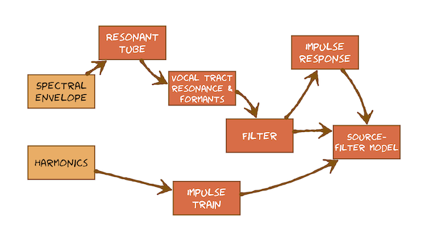
This video just has a plain transcript, not time-aligned to the videoWe now have all the components needed to assemble a computational model of speech.But, before we get into that, let's remind ourselves what the model will be used for.Well, lots of things!Primarily, understanding and explaining speech signals.But it has engineering applications.We could use it to manipulate speech.For example, we might wish to change the fundamental frequency or the duration, without changing the spectral envelope: that gives us a route to creating entirely synthetic speech.We might also use this model to extract features from speech, based only on the spectral envelope, without properties of the source, for use in Automatic Speech Recognition.The model is going to work in the time domain: in the domain of signals, but we're not attempting to model in detail the physics.We're working with recorded digital speech signals: waveforms.So this model is a model of the speech signal.Here are the key components.We've understood that the vocal tract has resonances: they are called formants.We generalised that idea to one of a filter.The filter was a linear filter: a simple equation operating in the time domain.We can characterise that filter in various ways.There's the coefficients of the equation, there is its frequency response, and there is its impulse response.If we take its impulse response and excite the filter with a train of impulses, we'll get out a train of impulse responses.That's the speech signal.So that's our source-filter model.Let's write down the full notation of our source-filter model.Here's a filter; it has some number of coefficients, p, called the order of the filter.We have to choose that value.I'm going to change from my earlier generic notation of x for input and y for output to some meaningful letters.I'm going to use e for 'excitation' (that's the input signal) and s for 'speech' (the output signal).We've already established the form of the filter.Here's a general equation; that's the same as the one we've seen before.This part used to be written '1.0 times the input' (for which we were using x).That's where that's gone.This part here is the weighted sum of previous outputs.This t-k is saying 'the previous output' when the k is 1, 2, 3, and so on on.We use p previous outputs.It looks a little odd to use k as the index term to count up to p, but that's the standard notation and I'm not going to deviate from that.So far, we've only seen the model generating voiced speech.We put in a periodic signal as the excitation: the simplest possible signal that has energy to every multiple of the fundamental, because that's what we see in speech signals.That simple signal is an impulse train.What we get out is the sequence of impulse responses overlaid on one another (because the filter's linear): that's our synthetic speech signal.So it's a model of signals.The input e is a signal: it's just a waveform.It's indexed by discreet time t because it's a digital waveform.e is entirely synthetic: it's something we will generate automatically.Let's watch the model in action, in the time domain.We simply write out this impulse train and we'll run that through this equation and get speech as the output.An impulse train is mostly 0 and then, just occasionally, there's a 1.That's the first impulse in our impulse train That will excite the filter and the output of the filter will, of course, be its impulse response.Instead of looking at this equation, let's look at the impulse response of the filter.In comes an impulse; the filter outputs its impulse response; that's the output.So we just write that on to the output.Because this impulse came in at time t = 5 ms, the output impulse response will start from t = 5 ms.On goes our input.Nothing happens...and then, some time later (another 5 ms later, in fact), in comes the next impulse.That also excites an impulse response from the filter, which starts at time t = 10 ms, and writes onto the output.We can see here that the second impulse response just overlapped and added to the first impulse response.Now, why did we just overlap-and-add that second impulse response?Well, that's what the filter equation tells us to do.It says that the output is just a weighted sum of the input inpulse and the previous filter outputs: it's linear.That linear nature of the filter tells us that the output is just a sequence of overlapped-and-added impulse responses.This whole process of taking this time domain signal and using it to provoke impulse responses and then overlap-and-adding them in the output is called 'convolution'.That process would work for any input signal.It could have other non-zero values anywhere.It could be a complete waveform of any sort we like and each sample would be treated like an impulse.It would provoke an impulse response which would write into the output.This idea of convolution is something will come back to later.Here we're using it to combine the excitation and the filter's impulse response to produce the filter's output.Understanding that process as convolution in the time domain is just fine, but convolution is a slightly complicated operation, so let's go to the frequency domain where things will look a little bit simpler.I'm going to synthesise this vowel.To do that, I just simply need to choose appropriate values for the filter's coefficients.Those values determine the impulse response of the filter.If we look at the Fourier transform of this signal, we get the frequency response of the filter.So let us now observe the source-filter model generating speech in the frequency domain.I'll put in my impulse train: there it is, with its characteristic spectrum with a flat spectral envelope and equal amounts of energy at every multiple of F0.This signal's going to go through the filter and produce some output.These magnitude spectra really reveal to us how this filter is operating.We take the magnitude spectrum of the excitation signal and it is multiplied by the frequency response of the filter to give us the magnitude spectrum of the speech.In other words, the slightly complicated operation of convolution in the time domain has become a rather simpler operation of multiplication in the frequency domain.This filter just has 4 coefficients - it's order 4 - and it has 2 resonances.That's a very simple filter.It's going to be a bit simpler than a real vocal tract.I've excited it here with an entirely synthetic signal - an impulse train - and so we can generate a synthetic speech sound.That's not great, but it has the properties of speech and you can probably hear that vowel.If we wanted to make a different vowel, we can keep the input the same.We could have different filter coefficients, leading to a different frequency response.Here it is.We will multiply this input magnitude spectrum by this frequency response to get the output, which looks like this.You can see that the resonant peaks are controlled by the filter and the harmonic structure is controlled by the source.That sounds like this.You can perceive a different vowel.Again, it's not very natural, because these are very simple filters with very simple input.We can keep changing the vowel by changing the filter coefficients, and its frequency response.Here's one more.That looks like this.Now, how about keeping the filter the same and changing the source?The source only has one thing that you can change and that's the fundamental frequency.Make it lower.Or make it higher.Hopefully you can perceive that only the pitch is changing and the vowel quality is the same.We've independently controlled source and filter.OK, that's enough vowels.This is supposed to be a general model that could generate any speech sound.So we better demonstrate it doing something other than vowels.Let's make an unvoiced fricative.To make this phoneme, we need to make a construction that creates turbulent airflow somewhere in the vocal tract.Then the part of the vocal tract that's in front of that - between that construction and the lips - acts as the filter and shapes that basic turbulent sound to make this unvoiced fricative.Just check that you can make this fricative.Pause the video.You made a constriction.You forced air through it to create a basic, turbulent sound.Then the remaining part of the vocal tract is the filter.We can model that with a basic sound of turbulence.This is a signal that is random, it has no periodicity but still has a flat spectral envelope.We call that 'white noise' because it has an equal amount of energy at all frequencies, like white light has equal amounts of energy at all colours.That's our simulation of the basic sound created by turbulence at a construction.Because there's less vocal tract between the construction and the lips than for voiced speech, where the sound source is right down at the bottom of the vocal tract, the filter is of a simpler shape.Therefore, we'd expect to see simpler spectral envelopes for filters in this case.With this spectral envelope - this frequency response - we can put white noise through this filter and make this sound [s].By changing the frequency response of the filter to this one, we can make a [sh].Now, it's all very well playing around with filter coefficients and with impulse trains and white noise as input, but it's never going to sound perfectly natural, and in particular, because the filter is a bit too simple.Everything you've heard so far was generated from hand-designed filters.I made them.I made up their coefficients to approximate some vowel sounds.That's very limiting.That's not going to be a good way to generate synthetic speech.Wouldn't it be better if we could take natural speech, like this, and fit the filter to it? Conceptually, that should be straightforward.We know the natural speech waveform, and of course its magnitude spectrum.So all we have to find is the frequency response the filter and the set of coefficients that has that frequency response.In other words, we have to find these values here.There are a variety of algorithms that will solve for those filter coefficients, given a natural speech signal.In other words, that will fit the filter to that signal.We're not going to go deep into those here.I'm going to fit a more complicated filter.I'm now going to ramp p up to a higher value of 24.That's why this has a more complicated spectral envelope than we've seen so far.But it still got peaks for resonances.I'm still going to excite this filter with an impulse train, so that part's still completely synthetic.This part has been fitted to a natural speech signal.By putting a synthetic impulse train through a filter whose coefficients have been recovered from natural speech, we can make synthetic speech that'll sound a lot closer to that vowel.The fundamental frequency is very unnatural, because it's monotonic.But the spectral envelope is the same as that natural speech we just heard.Now I can manipulate the fundamental frequency, whilst leaving the vowel quality alone.I can raise the pitch and I can lower the pitch.So, what have we achieved?We've taken natural speech, we've fitted the source-filter model to it, in particular we solved for the filter coefficients, then we've excited that filter with synthetic impulse trains at a fundamental frequency of our choice.We brought quite a few components together there, to make our source-filter model, but there's still a bit further we can go.Our source-filter model decomposes speech signals into a source component (that's either an impulse train for voiced speech, or white noise for unvoiced speech) and a filter (which has a frequency response determined by its coefficients).We've seen that we could solve for those coefficients, given natural speech samples.From now on, whenever you encounter something about a speech signal that you don't understand, come back to the source-filter model and try and use that to understand what's going on.We've understood our filter in the time domain and the frequency domain, and also in its coefficients - in its difference equation.In the time domain, its output, when we put in a single impulse, is called the impulse response.That's such a special signal, it gets its own special name in speech processing, and it's called a 'pitch period'.That pitch period is a fragment of waveform coming out of the filter, and that's going to offer us another route to using our source-filter model to modify speech without having to solve explicitly for the filter coefficients, because the pitch period completely characterises the filter.Eventually we're going to completely understand the process of convolution.That's the process by which the filter's impulse response combines with the filter's input to produce the output.That will give us another way to separate the source and filter called 'cepstral analysis'.We'll actually use that for Automatic Speech Recognition.The common theme that will keep coming back again and again is that speech is created from a source and a filter.The observed speech waveform - which is all we have as our starting point in speech processing - contains the properties of both of those combined.For various applications, we want to separate the source and filter.
This video just has a plain transcript, not time-aligned to the videoWe already developed the source-filter model, and we used it to understand speech production, and then we used it to synthesise speech.So make sure you've fully understood this model before proceeding, because now we're going to use it to understand what a phoneme is.Speakers have conscious control over many aspects of their speech.They can choose how and where to generate the basic sound, such as vocal fold vibration, or frication at a constriction.They can then modify that basic sound by passing it through the vocal tract filter, which they can vary the shape of.As always, a simplified model will help us understand that.So here's a reminder of the source-filter model.This is the filter, and it's most convenient to think about it (as always) in the frequency domain.So here is its frequency response.This particular frequency response has two peaks, which are modelling the resonances of the vocal tract: they're the formants.If we choose to excite this filter with a periodic signal - an impulse train that simulates the vocal folds - then we'll generate a voiced sound with this particular spectral envelope, and that will be a vowel.When the vocal tract shape changes, the formant frequencies vary, and the speech varies.We make a different vowel.By choosing an appropriate frequency response - in other words, appropriate formant values - a speaker can make any vowel they like.If we characterise this filter by these two formant frequencies, it seems quite natural to plot them on a chart with two dimensions: one for each of those frequencies.F1 is the first formant; F2 is the second formant.We've plotted vowel space, and this is clearly a continuum.By manipulating the shape of the vocal tract, we could make any value of these two formants that we like, limited only by the physical dimensions of the vocal tract: the minimum and maximum achievable frequencies.Try for yourself.Try making this vowel in this corner - that's [ɪ] - and then gradually change it to an [e].Pause the video.To make an [ɪ] vowel, your tongue has to be high in the mouth and forwards.To change that to an [e], mostly what you need to do is lower the tongue.So this dimension is to do with the height of your tongue in your mouth.Now, make the [ɪ] vowel again and gradually change it this time to an [ɔ:].Pause the video.What did you do that time?Well, mainly you moved your tongue backwards.So this dimension is something to do with how advanced in the oral cavity your tongue is.I've drawn this plot in a very particular way with the origin in this corner here.That's a bit unusual, but the reason for that is so these axes roughly correspond to the height of the tongue, and it's horizontal position, sometimes called 'front-back' or 'advancement'.That corresponds with the speaker facing to the left.That's why I've always been drawing this guy facing left, because it matches up with this vowel chart and that's how the IPA draws it.Vowel space is clearly acoustically a continuum.You can make any combination of the two formants limited only by physics.But it's linguistically reasonable to make these two axes discrete.That's because speakers can only control the tongue position with some amount of precision, and listeners cannot hear very small differences in the formant values.On the IPA vowel chart, there are 3 possible advancement positions and 4 possible height positions, which gives you 12 vowels.Oh, except for some in-between ones that don't quite fit that pattern.Oh, and except that also they seem to come in pairs, where one of them involves rounding the lips, which just makes the vocal tract a little bit longer.With the two dimensions of advancement and height, a third dimension of rounding, we could make an enormous number of vowels.No language in the world makes use of all of those vowels.I mean, imagine having to learn that language!But we'll come back to that in the video on pronunciation.That covers the vowels.The source-filter model is a very natural way to explain how we could make so many different vowels.Let's talk about some constants.In previous videos, we already made the unvoiced fricatives [s] and [ʃ].We did that by changing the source to a random number generator: that makes a sound called white noise.It has a flat spectrum, but no harmonic structure, putting that through an appropriate frequency response, and producing these fricatives.If we change the frequency response, we change the fricative.Our source-filter model has two possible sources: a periodic one and an aperiodic one.But why not have both at the same time?Make the sound [s] and then start vibrating your vocal folds as if you're also making a vowel at the same time.Pause the video.Yes, it's possible!What phoneme did you make?From [s] you made [z]Our source-filter model could do that.We're just going to add the two sources together before they go through the filter.This is great!We can have this source, or this source, or both.We can choose the frequency response of the filter.We can make lots and lots of different sounds.It seems that we can make almost any combination of the different features of our model and therefore create many, many different sounds.Here's the row of the IPA consonant chart for fricatives: look how many there are.We could make fricatives at every possible place in the vocal tract, from using both lips all the way back to the glottis.At every one of those places, we can either have voicing or not.How many of these fricatives can you make, from the languages you speak? Pause the video.I can only make a restricted range of these fricatives.I can make the ones from here to here.I can make [f] / [v] , [θ] / [ð] , [s] / [z] , [ʃ] / [ʒ].That's a lot of fricatives and we've got a lot of vowels, but let's keep going.There's more to speech than vowels and fricatives.There are more things we can control to make more combinations.If we can find just a few more things to control, then we'll be able to make even more combinations and make a lot more sounds.Here's how it works for fricatives.We make a constriction somewhere in the vocal tract, without completely closing it.We force air through.That makes turbulence - that's the source of sound - and that's filtered by the remaining vocal tract.By moving the constriction to another place, we can make a different fricative, because there's a different amount of vocal tract in front of the point of constriction.What about a whole different way of making the sound in the first place? Instead of making a constriction that produces turbulence, how about completely closing the vocal tract?Make a complete closure.Air is pushed up from the lungs and, just like at the vocal folds, eventually this closure will give way under pressure and burst open, and produce an explosive pulse of air that travels through the remaining vocal tract.Unlike the vocal folds, this process doesn't repeat: this is one-shot.We get a single plosive.Again, we can move that place of the closure to somewhere else in the vocal tract: maybe here.Air pressure builds up; we can't contain it; the closure bursts open, and we make a plosive sound.We can vary the place at which the articulation happens.We can also vary the manner in which that sounded is created.The manner of articulation of a fricative is to make a constriction and force air through a narrow gap.The manner of articulation of a plosive is to make a complete closure and then for that to burst open under pressure: to explode.That gives us another row in the constant chart, of plosives.There are lots of plosives - not quite as many fricatives, but still in many different places along the vocal tract.Like fricatives, many of them occur in voiced and unvoiced alternatives.In the consonant chart, the horizontal axis is the place in the vocal tract where the articulation takes place.The vertical axis is manner.'Manner' means the configuration of vocal tract created by some interaction between articulators: for example, contact between them.I'm not going to go through this whole chart because this is not a course on phonetics.This video is just to help you understand the connection between phonetics and the source-filter model, and how that model helps us understand how all of these different sounds could be created by combining features of the model.The story in this video, then, was one of contrastive features: a fairly small number of features, each with a relatively small number of possible values, that, in combination, results in a very large number of possible speech sounds.So many sounds that no single language uses all of them.Wait a minute!This video is called 'phoneme'.I have not actually defined the phoneme yet.All I've explained is how it's possible to make many, many different sounds.The real definition of phoneme has to come in the next video, in 'Pronunciation'.That's because it's language-specific.Each individual language has a phoneme inventory comprising just some of all the many sounds in the consonant and vowel charts from the IPA.The main purpose of the IPA is for descriptive purposes: for example, documenting a language, or writing down pronunciations of words.It's not quite good enough for generating speech, because of co-articulation.That's the way in which sounds are affected by their context.The IPA does not capture that in its symbols.Later on, we're going to need to account for that.In fact, not just in synthesis but also an Automatic Speech Recognition, contextual variation caused by co-articulation is a key thing that we need to account for in our models of speech.We'll encounter that for the first time in speech synthesis, where we'll concatenate fragments of recorded speech to generate new sentences.We won't concatenate recorded phonemes.We'll record units called 'diphones' which are in fact the units of co-articulation.From those, through simple concatenation of recorded waveforms, we'll be able to generate synthetic speech.
Reading
Wayland (Phonetics) – Chapter 6 – Basic Acoustics
A concise introduction to acoustics: sounds, resonance, and the source-filter theory
Handbook of phonetic sciences – Ch 20 – Intro to Signal Processing for Speech (Sections 6-7)
Written for a non-technical audience, this gently introduces some key concepts in speech signal processing. Read sections 6-7.
Johnson (Phonetics) – Chapter 2 – The Acoustic Theory of Speech Production: Deriving Schwa
Derives the acoustic features of the vocal tract in terms of the source-filter model
Johnson (Phonetics) – Chapter 6.1 – Tube models of vowel production
Deriving the resonances and formant structures of vowels using 2 and 3 tube models of the vocal tract.
This is a SIGNALS tutorial in which you will work with speech signals.
These labs follow on directly from those in Module 3 (Digital Speech Signals). You can find info on how to download and get started with Jupyter Notebooks in the Module 3 lab tab.
You can find a github repository for the signals notebooks here: https://github.com/laic/uoe_speech_processing_course. You can find the notebooks for this module in that repository under signals/signals-lab-2.
Some of the notebooks you’ll find there are essential and some are extension material. Your task for this week is to go through the notebook marked essential, relating to the Source Filter model:
The other notebooks in that directory give some mathematical extensions on the essential materials. You can find a list of more notebooks in the overview notebook here: signals-0-start.ipynb.
Answers/Notes for Module 4 lab
The source-filter model of speech gives us a way of writing down the generation of speech sounds in the vocal tract in mathematical terms. Here we modelled the source as either a series of impulses or as white noise, and the filter in terms of Infinite Impulse Response (IIR) filters.
You will have seen in the labs that interpreting specific IIR filter coefficients in terms of resonances is not at all obvious. We don’t go into the details in this class, but this is a case where viewing what the filter in a transformed representation (in this case, the z-domain) makes things more interpretable. This requires quite a lot more mathematical scaffolding, which is why we don’t go into it here. In general, signal processing is an area with well developed mathematical tools which make determining a filter’s actions on a signal much more transparent. Understanding this can be very important for improving signal quality in different real life situations, but that is beyond the scope of this course.
The important point to take away is that once we know the frequency response of a filter, we can easily determine what it’s effect will be on a signal will be. In the case of an impulse train, the filter’s frequency response (magnitude spectrum) will be superimposed on the frequency response of the impulse train, causing a change in the spectral envelope. The fine detail of the spectrum will be determined by the fundamental the fundamental frequency of the impulse train and integer multiples of that (harmonics).
The idea of extracting well-behaved features that compactly represent the spectral envelope of speech sounds through time will lead us to the concept of Mel-Frequency Cepstral Coefficients in Module 8. These sorts of features are the backbone of most Automatic Speech Recognition Systems and statistical Text-to-Speech systems. In the next weeks, we’ll turn our attention to concatenative speech synthesis, where we’ll look at generating speech from text inputs based on the acoustic properties of speech units in a speech database.
What you should know
Spectral envelope, Resonance, Vocal Tract Resonance:
- Describe how we can approximate the vocal tract in terms of a series of tubes (i.e. physical source filter model
- What’s the source? How does it relate to F0
- What determines the filter properties? How does this relate to resonance?
- You won’t be expected to derive any actual tube models for specific vowels or do resonance calculations.
Harmonics, Impulse train:
- Explain what an impulse and impulse trains are
- Explain how we can determine/change what fundamental frequency and harmonics of an impulse train will be
Filter, Impulse response, Source-Filter model
- Describe the difference between a Finite Impulse Response (FIR) and an Infinite Impulse Response (IIR) filter
- Describe the relationship between resonances, the spectral envelope of a sound, and the frequency response of a filter
- Explain what represents the vocal source in the source-filter model, and how this can be varied to represent different classes of speech sounds
- Explain how the vocal tract resonances are represented in the source-filter model, and how these can be varied, and how these relate to our perception of speech sounds, e.g. in terms of formant structure
- Describe the difference between low-pass, band-pass, and high-pass filters in frequency domain terms.
Extensions
The version of the source-filter model presented in this course works pretty well for a broad characterisation of some phones as presented, but you’d be well justified in wondering whether it’s an oversimplification of the vocal tract (e.g. where’s the nasal cavity in this model?). A classic text on acoustic phonetics is Ken Stevens’ Acoustic Phonetics. This is well out of scope for this course, but a quick browse of chapter 3 (‘Basic Acoustics of Vocal Tract Resonators’) which give you an idea of the complexity involved in modelling more detail in speech production.
If you want to try to build your own physical tube model, Mark Huckvale has some practical instructions here.
If you’re interested in learning more about filters or signal processing in general, I recommend Rick Lyon’s Understanding Digital Signal Processing as the most accessible yet mathematically clear textbook on this area I’ve come across (unfortunately, the University of Edinburgh library only has paper copies on short term loan). Previous SLP students have also recommended The Scientist and Engineer’s Guide to Digital Signal Processing by Steven Smith, which available for free online. Again, going further into Digital Signal Processing is out of scope for this course, but you may well find a bit of extension useful if you intend to pursue this line of study in the future.
Key Terms
- Spectral envelope
- Resonance
- Vocal Tract
- Formant
- Source
- Filter
- Difference equation
- Impulse, Impulse Train
- Impulse response
- Finite Impulse Response
- Infinite Impulse Response
- low-pass, high-pass, band-pass