Module 10 – Speech Recognition – Connected speech & HMM training

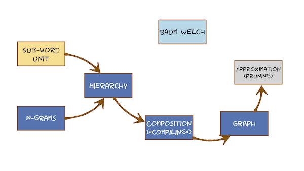
This video just has a plain transcript, not time-aligned to the videoTHIS IS AN UNCORRECTED AUTOMATIC TRANSCRIPT
A LIGHTLY-CORRECTED VERSION MAY BE MADE AVAILABLE IF TIME ALLOWS
This is the last module of the course module.
Nine actually got two parts to it.
The first part's actually quite easy connected speech.
Surprisingly easy on the second part's quite hard on our final destination.
Off Rachman training will be the Bond Welsh algorithm, which is conceptually the hardest part of the entire course.
So looks like there's an awful lot to cover in this module, but the individual videos are pretty complete, and so this is really going to be just a no overview to join all of that together and show you how the individual videos fit into this topic map.
These are topics have actually covered previously, but we're going to see them link back in now and help us get towards our final destination for hmm, training the bound Welsh algorithm.
Before that, let's just deal with connected speech, which is surprisingly easy on.
We've made it easy by choosing to use finite state models, and we're going to keep choosing finite state models, and everything will compile together into a single graph that will just be another hit of Markov model.
We're motivated Hmm Tze from pattern matching, but I think we can get beyond that now so we can treat a gym moms as a model in its own right.
It's a finite state model, so it's made of a finite number of states.
Joined together in the network with transitions in each of those states is a Gaussian probability density function whose job is to emit observations on DH so the model is emitting or generating on observation sequence.
It's a probabilistic generative model, so we moved on now from pattern matching into thinking always in probabilistic generative models.
On the key point of the model is that you can capture the variability that's present in natural examples of speech.
So it learns from data so the model accounts for their ability, and it does that at the core by using probability density functions.
Pdf ce on.
We're going to use gas.
Ian's, the finite state.
Part of the model is simply there to specify the sequence in which to use those pdf ce so the model is a generative model generates sequences.
So for that reason, our M SEC vectors we now refer to ours observations because they are the observed output of a generative model.
When the model generation observation sequence.
All we see is the observation sequence.
We don't see how the model did that.
Specifically, we don't see that state sequence the model took.
That steak with sequence is hidden.
State secrets is just another way of saying the alignment between states and observations many possible states equals is Khun Generate the same observation sequins each state.
Secrets will have a different probability of generating the observation sequence, but there be many non zero ones on that arises because of Gaussian Khun.
Generate any observation with non zero probability Galaxy in assigns a non zero probability or, strictly speaking, probability density, tow any value in practise.
When we doing inference with the model from using the model to do pattern recognition to do speech recognition, we can get away with only considering the single most likely state sequence.
There's an exact algorithm that finds that one most likely state secrets called the Viterbi algorithm, and that's what makes speech recognition fast and efficient.
But now we need to revisit the definition of the model and see that this approximation of using the most likely state sequence needs to be replaced with a sum over all possible state sequences because when we train the model, we can't a lot less about speed are much more about getting the best estimate of the models parameters.
So let's get on with the first part of the module, which is the easiest part.
And that's the deal with connected speech.
And then we'll come back to this idea ofthe training a model.
A lot of the language with you so far about hidden Markov models is involved, saying things like There is a model for each class that we're trying to recognise.
Typically, those classes have bean whole words, and we assumed that we would need to do separate computation for each model to compute the probability that it emitted.
The given observation sequence that we tried to recognise would repeat that a number of times one time for each word in Africa.
Bricks of 10 times for our digit.
Recognise er compare 10 numbers.
Pick the highest and label.
The observation seems with that class, that's fine.
That would work, but that's hard to see how that might extend to sequences of words.
So we're now going to introduce language models.
Language models will allow us to account for the pride probability off a word or of a word sequence.
And now we'll be able to move away from saying we compute 10 separate models to combining them in a single model.
That's where we're going on our solutions.
That is going to be an engram.
So the solution to worse sequences this to create a model, often utterance, that generates words.
Everything is a generative model.
Let's just recap how an Engram language model works.
So in the end, Graham, we have to choose the value of N a popular choice might be to for by Graham three for a try a gramme and maybe higher.
If we have a lot of data, let's draw a three gramme or try Graham in an Engram language model.
There are a number of states in the states, a label with word history.
So in a tri Graham language model, the word history is the previous two words.
Are we getting the probability of the next word? That's where n equals three comes from, and so we label estate with history, so he's going to some number of states, and if we had em words in our recovery going tough, M squared such States in a tri Graham.
I won't know them or because if M was, thousands would have millions of such states.
Let's just draw few examples.
Ones here is one where the word history is the cut.
Any arc coming out of that state is going to be the probability off the next word given history was the count.
Maybe next word might be SAT is quite a likely word, but would have one art for every possible following word.
So we've got the cat in the history and sat being the thing we're predicting the probability off that we generate.
The word sat as we move down this ark.
History now slides forward, so the history now becomes cut.
Sat on.
The has dropped off the end because it's outside the Engram now and is only three.
So the window of histories to any are coming out of here.
Going to be the probability off some word given cut sad.
And so we'd put anywhere you like in here and predict its probability and so on.
So the states were labelled with the word history.
It arcs have the probability of the next word.
Given that word history on out of every state to be lots of arcs, going to all the possible next words.
So if this was a complete model that b m such arcs, because any word could follow this history and principal with a non zero probability on this model would have a size that's governed by the vocabulary on DH by N if n got larger.
If instead of a trial Graham, we attempted to build a four gramme.
Each state will be labelled with the three word history, and we would now have not m squared.
But M Cube states so we can see why we very quickly have to keep n under control on the three Grand was already got a lot of states of four grammes going to have a huge number of states.
It's very rare that we might see anything bigger than four, maybe five, Grammys about our limit.
It's not that the model is too big.
Is that the number of parameters the model house is too big on.
Those parameters have to be estimated from data by counting these words sequence occurrences in some corpus.
We're not going to do the training of Ingram's in this course think intuitively, Khun.
See that? That would be very straightforward.
We would just count how many times sat followed the cat, and we count how many times any other word here followed the same word History on normalise it and get a probability from that.
That would be a simple way to estimate the probabilities of this engram for our purposes.
The most important property of the Ingram language model is that it's finite state.
There might be a large number of states, but there's a fixed countable number.
It's finite.
That's the solution to connected speech.
To make a model that emits word sequences, we took a random walk around.
This end Graham language model would emit random sentences.
The second problem we have if we want to do large recovery connected speech recognition is that the recovery might be large.
We need to define it in advance.
We want to specify the words that I recognise her will recognise on DH.
We don't want to be restricted toe having many examples of each of those words in the training data that will be very restrictive, and it will prevent us from ever adding a word to our recognise her without going back and getting Mohr recorded speech.
We don't want to have to do that.
If we got the covers of tens of thousands of words, we can't guarantee that every one of them occurs enough times in the training data, so we simply can't use whole word models.
The solution to that very obvious.
It's exactly what we did, what we did speak synthesis.
We didn't con continent recordings of words we can caffeinated recordings of phone, name sized things and speech synthesis.
Those were die phones.
Let's start with something very simple for speech recognition.
The phoney ins themselves will make models off phone aims.
The solution is of the same form as for speech synthesis.
Use of word models on DH phonetics tells us the appropriate so would unit to use.
And it allows us to write a dictionary, which is the mapping from words to phoning sequences by hand in the same way we we would do for speech synthesis.
So to the Ingram solution for connected speech, we have the solution for larger recovery, and that's to use a word units.
But everything's a generative model, so this is also a generative model going to have a generative model off a word.
Let's have general model of this Ortho graphic word cat.
That's the spelling of cut.
And it's going to be finite state like that now it doesn't really matter.
In finite state, formalism is whether we label things on states or arts will move through them all.
There are different formalism.
Is that possible? We saw in the final state transducers for speech synthesis that all the action happened on the arcs in the States.
We just call them the memory we saw in the Engram language model.
Those probabilities are on the arcs, and the states are the memory of the history.
Hear of drawn four names on the states that could equally have drawn the monarchs joined together with states.
That Ridge is a matter the point again that this is a finite state model off the word cat.
Given the Ortho graphic word it emits, it generates the sequence of phoney names.
We've got things happening, a couple of different levels there.
We got sentences made off words.
Sometimes we use the word utterance rather than sentence.
Just to be more general sentence implies some grammatical structure spoken language isn't always grammatical, so we use the more general term utterance utterances made off words.
It's the secrets of words.
A word is a sequence of phoney names.
So there's some hierarchy in learning language on DH described that very simply, we can solve the problem of large recovery connected speech recognition with this hierarchy of models, which combined will give us a generative model of a complete utterance.
First, a generative model of the veterans emits a word sequence each word In that sequence, a generative model of that word emits a phoney, um, sequence that models created from a dictionary.
I would say that that model is the dictionary, and then, for each phoney we have a hidden Markov model on that emits an observation sequence.
Generates the acoustics off that phoney no borders, No.
In the assignment we don't have.
Phoney models were committing this step here, and we have a generative model.
The entrance that emits a word sequence on a generation model of each word that emits an observation sequence That's fine, too, is still a hierarchy.
It's just, um, it's one of the levels.
So this hierarchy of models that all finite state or we need to do is to divine how to join them together.
The technical term for that in finite state machines is composition.
We're going to use another term compiling.
That's the terminology often used by H.
D.
K.
For example, how does that work? So this is only going to be possible if all the generative models of finite state combined them together or compose them in a finite state.
Model terminology to make a generative all oven utterance that emits acoustic observations emits, MFC sees the normal terminology in the field is not really to talk about an entrance model.
We call that the language model, for example, the Engram written as a finite state network instead of talking about word model.
We just don't talk about the dictionary Pronunciation dictionary on the sub word model.
We call it the acoustic model because it's the part of Modern.
It finally actually emits em of CCS or whatever Observation vector.
We've chosen composition in finite state models, Khun mean quite a lot of different things, and this is not a complete course on finite state models, so I'm only going to define the sort of composition that we're interested in here, and that's this hierarchical way of doing things.
Think ofthe part off our model that's keep things simple and have on utterance model where the states had just labelled with words.
We could think ofthe replacing that with this model.
And then we can think off replacing each of these things with I had a Markov model, and now it's obvious why we like HD Kay's way of having non emitting starting in states because they're convenient places which to glue together all these different models.
So composition here means to replace a model ofthe word to get this and then for that, replacing each phone aim with its generative model.
It's acoustic model.
That's an operation that's happening on a finite state network.
It's not a transducer of the form we saw in speech synthesis.
It doesn't have input and output.
It just generates on.
If we remember the path we took them, we can recover the most likely sequence of models and use that as the output of the system.
The resulting structure is a finite state model, and I'm going to call it the graph, but as well about see, it's actually just one big.
Hmm.
So we'll have always Cem well defined place to start.
Listen, what? And we're going to have a big, finite state network, which is the composition off an Engram language model or any other finite state model, perhaps one drawn by hand in the case of a simple digit recognise er Ingraham language model.
A dictionary on DH acoustic model through one of the phoney names on DH after the compositions happened after the compilation has happened, we just get this big graph and it's just on.
Hmm.
So we might have some non emitting states, some emitting states, nonentity states from committing states and so on and so on.
Once we've made this graph, this composition process is finished.
All that we have is an hmm.
This is Justin.
Hmm, More complicated looking than some of the H moves you've seen before, but it's got nothing in it that's different.
It's only got some non emitting states that just do the glue.
It's got some emitting states that will admit observations every time we visit them.
It's got some transitions which are part of the H M M's some transitions, which are joining a gym.
Moms together some transitions which are coming maybe out of one word and into the start of the net.
Next word and so on.
It doesn't matter for the purpose of computation where each of the transitions came from, because the whole thing is just an hmm, some of them may be.
This one might be the probability from the language model.
Some of them might be self transitioned on, Hmm States there from the acoustic model.
None of that matters because if you understand token passing, you put a token here on just press go on the token passing algorithm on DH at the point that you generate all the observations.
Look at what token comes out to the end state of the exact time.
And that's the winner Northern needs to do is to remember the sequence of models it went through, or at least to remember each word that it went through.
And that will be the recognition output.
It's really that simple.
There's nothing more to say.
The algorithm is the same on this network as it will be on a small, simple Hmm.
The hasty Keitel H.
Right does explicitly this in software.
It composes it compiles this graph and then it does token passing on that.
It's a token passing on that graph is just a practical implementation ofthe dynamic programming because we're doing on something that's a hidden Markov model.
We call it the Viterbi algorithm so we can do the Viterbi algorithm on that graph.
That graph, as I just drew it, is the same as the picture of the hmm.
It's drawing like this, the one that's the finite state picture oven.
Hmm.
There's no explicit time Access was very careful not to think of this having time flowing from left to right.
It's just a finite state model because we could have transitions like this, and that's perfectly legal.
That graph is the finite state picture off the model for speech recognition.
We can do Donna make programming on that directly on that data structure.
The implementation of that is called token passing.
As soon as that Graff gets reasonably large, we will want to do some pruning.
I'm pruning is an approximation, so the Viterbi algorithm is an exact algorithm.
It will always exactly find the most likely state sequence through.
The model will find the same one every time and it's not an approximation.
But to do that, he has to consider many state sequences on.
Many of those will be pretty unlikely a lot of the time and so we can make that would go a lot faster by pruning away by discarding some paths.
So if you see the little video about token passing, here's a screenshot of it.
At this moment in the algorithm, there are a lot of tokens alive.
The algorithm has been running for enough time, steps of emitted, enough observations that talks have propagated throughout the whole model.
But some of these tokens will be very likely they are likely to end up being on the best path they have.
A good chance of being the winner on others might be very unlikely.
We might be willing to take a small gamble and say they're so unlikely we don't think they'll ever become the winner.
We can't prove that we can just guess it, and we guess that they won't become the winner and will discard them.
Now we'll delete them.
So imagine we delete that one there.
This is an approximation.
If we do too much of this, have to do too much pruning.
We will eventually delete tokens that would have gone on to be the winner without knowing it, because we haven't finished the computation.
But normally we could do quite a lot of pruning without taking much risk.
That pruning will make computation much faster because we are massively reducing the number of tokens that we need to propagate each time step.
We think about some big graph, some very large number of hmm states.
Most of the tokens will have a very low probability.
How do we define whether they're too low? How do you define which took us to prune? Well, we just find the best token at that moment in time, we define a probability that some distance below that some threshold on that amount is often called the beam.
So this is beam approving, and we discard all tokens that outside the beam that the lower probability than that beam that finishes connected speech we form an utterance model, which is an engram, emits words for each word.
We omit phone aims.
That's a hierarchy of models.
We joined them together through a process which might come formally call composition, but well, more informally called compiling.
That's what H D.
K uses would compile a graph.
Sometimes call that the recognition network.
That's the thing on which we could do token passing directly on that data structure and that will perform the process off recognition that is an implementation of the Viterbi algorithm for hidden Markov models.
If the grafts reasonably large will want to speed up that computation by discarding very unlikely path before they've propagated all the way through the model, that's an approximation that's a process known as pruning.

This video just has a plain transcript, not time-aligned to the videoTHIS IS AN UNCORRECTED AUTOMATIC TRANSCRIPT
A LIGHTLY-CORRECTED VERSION MAY BE MADE AVAILABLE IF TIME ALLOWS
Let's get onto the harder part of this module, and that is how to train hit a Markov models.
So H bombs have a hidden state sequence.
Nuts.
What's fundamentally going to make the algorithm hard? We've seen that we can express the hidden state sequence by drawing out the lattice, and that's unrolling the hmm over time to show the hmm states exist in all times.
On.
That expresses the fact that there's many possible paths for recognition, for the process of doing inference with the model to find the most likely words.
Given the observations, we often only care about finding the most likely path, which is an approximation to the sum over all paths.
Once we've decided that approximations fine, we can use an exact algorithm to find that path.
So don't confuse the fact that finding a won best path isn't approximation to summing over all paths with exactly finding that one best path correctly.
So, knowing all of that, we're now going to derive a method for training.
A model mother was finding estimates of its parameters, given the data, and that's the bound Welsh algorithm to warm up to the bound Welsh algorithm, which is conceptually hard on DH.
We are only going to go for the concepts of it.
We're not going to work detail about the mouth that's in the readings to warm up for that, let's just recap this very famous equation that we should now understand on the left off this equation is what we actually want to compute for every possible w in the language.
So all the things that the person might have said when speaking to our speaks recognise er we want to compute the probability of each of those given the sequence of observations have arrived at our speaks, recognise her, and then we'll pick the W that maximises this term.
We can use Basil to rewrite that as the terms on the right.
We can write the probability of the observations, given the words.
That's the thing called the likelihood.
It's what our hmm computes multiplied by the probability of just the words.
There's no observations have been involved in that term, so that must be something you can compute without any observations.
In other words, you compute it before you see the observations, and that's known as the prior.
It's your prior belief, or your biases over which words are words.
Sequences are more or less likely that the language model on this unfortunate term here is the pride of probability of a particular observation sequence, which we have no idea how to compute.
But we don't need it because for anyone run of the speech recognition system, always a constant, soapy Evo is a constant, and so we typically cross it out.
Right proportional sign in here.
And don't worry about this term.
If we multiply together, the likelihood by a prior what we get is the probability after seeing the observations on the fancy word afterwards is posterior behind.
And so that p of W given those afternoons, the posterior.
The basing way to read this equation is to say that our prior beliefs about W before we made any observation, have Bean revised by receiving some evidence.
Given our prior beliefs, we received evidence.
Oh, we've revised our beliefs about W by multiplying the likelihood by our prior and this is our revised beliefs about W p l w not condition on anything.
That's our advanced belief.
What we believe before we hear anything language model, and then we have our POW.
Given some observations, that's the posterior after we received the evidence.
So we can think of this as a way off.
Revising beliefs, belief, revision so hidden stay sequins causes us problems.
Let's define some terms.
We want to compute the probability of a sequence of observations.
Given the model, we can compute two things.
The correct thing to do is to consider all possible state sequences.
We often use the random variable cue to refer to the state sequence.
Consider all possible state secrets is.
Q.
We marginalise Q away, and that involves summing over.
Q.
So we sum over all possible state sequences to give the total probability that the model emitted the sequence of observations that probabilities sometimes called the Forward probability and the algorithm for computing.
It is unsurprising, he called the forward algorithm.
That's the correct computation to do with hmm, because that could be expensive because it's a lot of things to sum up there.
We often approximate the forward probability with just the probability along the most likely state sequence.
So we just take a single most likely value of Q.
We search for that.
It's a search problem.
The Viterbi algorithm is the solution to that problem.
The Viterbi algorithm finds the most likely Q the one most likely.
Q.
We approximate the sum, the forward probability with the sum just along that Q.
And that's like taking the max.
This would appear to be the correct thing to do to do automatic speech recognition.
It is by definition, of the model, however we find in practise.
This works at least a CZ.
Well, there's a lot faster.
So the Viterbi algorithm is the default for doing inference for doing automatic speech recognition once the models being trained.
What we're going to talk about now is how to train the model, how to estimate its parameters, and we'll see that we need a more complicated album for that estimate.
The promise, the model given on observation sequence that we know came from that model.
So the data and labelled and that's the forward backward algorithm.
So we're just going to work our way up to that conceptually, and we'll finish by just seeing what it would look like to do the computations for the forward backward algorithm.
We leave the mass for the readings.
You'll never be asked to reproduce those math in an exam situation which want to get a conceptual understanding of how we would train this model.
All of these algorithms involves something like dynamic programming, the Viterbi algorithms and explicit form of dynamic programming.
But the forward algorithm and the forward backward algorithm also have ways of being extremely efficient weaken some over a very large number of possible state sequences in the most efficient way possible.
So the key property of the hmm that hope we understand by now is that I show you this model and I show you this observation sequence Exactly how that model generated observation sequence is known only to the model.
It's not known to us.
We observe the observations.
We don't get to see the state sequence.
You want a mental concept of this model emitting this observation sequence? The way to think about that as a Beijing would be to have the model emitting in all possible ways at once simultaneously.
So the model simultaneously does that on DH that on DH that and so on and so forth.
Every possible permutation off state sequence that could generate this observation sequence.
It's doing all of them once, and they have very improbabilities.
Those are just some of the many possible state sequences for this three emitting state model on the sequence of 66 observations.
Another view of the same thing now for a bigger model on the longer observation sequence is not to see the finite state machines is to look at the lattice.
And so now we don't need to draw sequence result on top of each other, because this shows us, all of them.
Let's just draw some paths through this lattice by which this, hmm, could align with the sequence of observations.
You know, there was that it could admit the sequence of observations.
Not all parts of this lattice here are reachable because off the topology of this.
Hmm.
So this part is reachable in this part.
These useless because we can't get to the end.
We have to finish here in this particular model will start here on these we don't ever get to from the start.
So this area here expresses all the different paths through this.
Hmm.
Could generate this observation sequence under all of these joined up.
So therefore, lattice, look something like this.
Sometimes people say trellis instead of lattice.
I think those people must be gardeners.
This lattice is a picture off the hmm emitting the observation sequence whilst taking all possible paths.
Benjamin was a very simple model.
It has no memory.
The state is everything.
So we say the state is the memory.
There's no external way to store any information.
So anything that model needs to know is encapsulated by being in a particular state.
What does that mean? In practise? Let's consider this model generating this observation.
Sequins on DH Being in this state when we generate this observation sequence, imagine this's part off the way that this model generated this observation sequence.
Knowing that means that how it generated this part of the observation sequence is entirely independent of this because we know the current state to the past in the future become independent, given the current state.
So we say they are conditionally independent.
What does that look like on the lattice? We'll zoom into a particular state.
That's now this state, anything.
This observation in the sequence that means that all the computations to get to that point which involved all of these paths here are conditionally independent off.
They have no bearing on the computation off how to get from the state to the end.
The green computations on the purple computations are entirely independent.
They could be done separately, for example.
The model is mark off its memory less.
Another way of saying that is all you need to know is what state you're in, not how you got there.
So if I say that we're in this state than the probability off this state admitting this observation depends only on that state.
In other words, what gal scenes air in there.
And most importantly, it doesn't depend on how this observation was emitted.
It could have also come from that state.
But we've forgotten.
Or it could have come from that state with forgotten.
And it doesn't depend on how are we going to generate this observation, whether we're going to stay in the same state or whether will have moved to the next date.
We don't need to know that the probability of an observation depends only on the current state.
So what we say is that the observations are independent of each other, given the state.
So we're not saying that observations are just independent of each other.
They're independent, given the state, so they are conditionally independent.
That's not quite such about assumption.
We're saying that all you need to know is this state.
What that means when we doing computations on the lattice is that if we have arrived here, we want to find the probability of admitting this observation.
Everything we need to know is locally is contained here.
It's in the guardians for this state.
We don't need to remember how we got here.
We don't.
You know how we're going to leave.
Computations happen locally on that simplifies computation enormously.
So there's the key properties oven.
Hmm.
So now what's the computations do we need to do to be able to train such a model? Let's just recap the one that we do recognition with.
That's the Viterbi algorithm.
Well, when you put a token in the start, I'm run tau comm passing, so we wantto comm passing at some point token comes out the end.
Having generated all the observations in the sequence is token.
If we wished could record it state sequence and we could recover that and tell us the one best state sequence.
That's one computation we need for the Hmm? What is that look like on the lattice? Well, he just finds us one path from start to end, for example, it might find us this one and no others.
And it'll tell us the probability of the model generating the reservation sequence and taking that one state sequence.
And that's what we used to do.
Recognition.
If you want to exactly compute the total probability or this model emitting this observation sequence, we need to sum over all state sequences.
We need to marginalise out the state sequence, and that will be to do the correct computation to do this some and not the max.
And that's called the forward algorithm.
This becomes harder and harder to understand on this finite state picture much easier to understand on the lattice.
So again, let's just draw the part of the leftist that's actually reachable for this particular model topology.
In this particular observation sequence on, we're now going to some across all paths through this lattice.
Into that summation.
Let's just pick a place where we doing some of that computation.
When we arrived here, with some path coming in this way, the bath coming in this way.
Plus the probability off emitting this observation, Who some of these probabilities together, Write it there and then that propagates forward through the lattice.
Until here is the total probability of going from the start to the end and emitting the observation sequence using all possible sequences.
So summing away Q.
You could do recognition with that, and you would use the probability here in the final state as the final probability, the total probability that this model emitted this observation sequence.
So now the hard part, the bound Welsh algorithm in the Bow Marshall gone.
We're going to have to compute something more specific.
And that's the problem with being in a particular state at a particular time.
And we'll need that to know whether that state emitted a particular observation or not.
And if we knew that, we could use the observation update that states calc ins

This video just has a plain transcript, not time-aligned to the videoTHIS IS AN UNCORRECTED AUTOMATIC TRANSCRIPT
A LIGHTLY-CORRECTED VERSION MAY BE MADE AVAILABLE IF TIME ALLOWS
going to get to the bound Welsh algorithm through so much simpler training methods.
And if you only ever understand these simply training methods, that's fine, because the second of them Viterbi training, works pretty well.
Ideally, for the course.
I want you to get at least a conceptual understanding of how to get from Viterbi training up to the full bound Welsh algorithm, trying to sound the maths from the readings if you can.
But if they're beyond you, at least try and get the concept that we're moving from one best path toe all paths from one best state sequence.
Allstate sequences.
Thies, too.
Simple methods are used, and in fact, both of them are on one after the other in the assignment in the tool called H in it.
Now, you won't able to tell it in the assignment because the data so small and the models are very small.
But agent it is very fast, and then Bam Welch is used as a follow on to that to initialise the models with these very fast algorithms that aren't quite perfect.
And then we run down Welch in H rest, we'll re estimation, runs the bound Welsh algorithm.
We run them in that order.
These simple methods make a hard alignment between observations and states.
In other words, anyone observation in our training data is aligned with precisely one state in the model, and it contributes only to updating the galaxy in in that state when we update the model parameters.
One way to describe the bomb Welsh algorithm slightly vague way is that there's a soft or probabilistic alignment between observations and states.
In other words, on observation in the training data could have potentially being emitted by one of quite a number of states, potentially any state in the model.
And it could therefore contribute to updating the parameters of all of those states to varying degrees, depending on how likely it was that it came from that state.
That it was emitted by that state.
Slow start with simple methods to simple training methods.
First one is called uniforms segmentation.
Here's the sequins off.
Six observations were gonna consider training a model only on a one observation sequence for now, and we'll worry about multiple sequences in a moment.
We got six of them.
We've got three emitting states.
The obvious, rather naive thing to do just to divide them up, take the mean of these two and write the mean here, take the variance, and that's its variants.
These ones they used to update this won on these ones are used.
Update this one done.
There's no point repeating that because you got the same answer every time.
That's called uniforms segmentation.
That's pretty easy to understand on this finite state picture.
But let's do it on the lattice because it will help us get to the bottom Welsh algorithm, which would be just too hard to draw on the final state model.
What did you inform segmentation look like? We've got 1234567 10 11, 12 13.
Observations are sequence.
We got five states.
It doesn't divide uniformly, but there's going to be about three observations per state.
So we're going to take a path through the lattice, which is the closest to diagonal that we can.
You have to just do some rounding so we maybe go give the first three to that state on three two, and then three and then, too.
And that's just like saying thes.
Three observations going to contribute to this calcium, so that's uniforms segmentation on the lightest.
Just take the most diagonal path that you can, given that you couldn't interview number off observations and an interview number of states.
There's only one such path.
So you just take that one and update the mobile.
Let's go back to the finance state model for you for a minute.
We can always find a better alignment between the states and these observations on the uniform one, and that's by doing what we do it recognition and using the Viterbi algorithm.
Now the Viterbi algorithm is only going to work.
If the model already has parameters, you form segmentation Khun work.
Even the bottle has no parameters because the model primitive have no influence.
On the alignment is just the number of states and number observations that matter.
So we use uniforms segmentation to give the model some parameters.
Given those parameters from the Viterbi algorithm to find an alignment between states and observations, possibly this one in general, this will be different to you.
Form segmentation will use this alignment, update the models parameters.
The model promises have now changed, and they're for if we run the Viterbi album again we make a different alignment, so maybe next time we'll get misalignment and will update the model promises again.
I will repeat that until the model stops getting better.
We could think of that until the alignment settles down to something stable.
But in fact, what we measure is the probability of the observations given the model and when that stops getting better determinate the algorithm.
So this is attractive, given the model parameters we find in alignment.
We use that to update the model model has changed.
We find the next alignment, which should be better because the models got better and we repeat that until it stops getting better, ones that look like on the lattice.
Well, now, rather than just finding the most diagonal path through the lattice, we actually do dynamic programming.
So off we go do dynamic programming.
Maybe it finds a path through the lattice like this.
We used that alignment to assign these observations to this state.
These observations to this state, all of these observations to this state and so on.
Then we just repeat that until the model set stops getting better.
So that's two very simple methods of training them all uniforms.
Segmentation is not intuitive because you got the same answer every time, so no point running it twice.
It's fast.
It's very approximate, but your model gets some parameters that are better than nothing better than, for example, giving them uniformed parameters.
In all the states, you've got an approximate model.
You then use that as the starting point for Viterbi training.
You do a few alterations off Peter be training, realigning the model with the data until the model stops getting better.
And then you got a trained model trained with a Viterbi algorithm before we move up to the bound Welsh algorithm going to talk about something else.
And that's how do we use multiple training examples? So let's stick with Viterbi training, where we find on a line between a model at an observation sequence and then update the model.
So let's assume that I've used uniforms segmentation to initialise my model.
So this picture is the same model six times, aligning itself with six examples, six training examples.
So let's imagine this is a model off three on DH.
We got six recordings of the word 31 model.
We want to estimate this model on these six recordings for each training example.
So that's training.
Example.
123 for five and six have recorded it six times will perform Viterbi alignment to align the model with the observations.
That one was easy.
This one maybe would find this one and so on.
So we do.
Viterbi are going to find these alignments, I imagine that's what my Viterbi algorithm finds me for the six different recordings of three but the one same model.
And now I update the mole by averaging across all six repetitions.
So this state aligned with this observation this one, this one, these two this one and this one nuts.
123456 There seven observation factors there.
So just sum them up, divide by seven, and that will become the mean of that state.
And we'll do the same for variance and for the means of Aristotle.
The other states, when we train on multiple training examples, multiple observation sequences, we simply do the summing and the averaging over all of them, rather just within one sequence.
The extension is very straightforward.
So for the rest of the explanation, I'm going to just revert to training on a single observation sequence because it makes the explanations much easier.
But the extension to multiple observation sequences is easy.
Any summation we did within observation sequence, we just extend to something across observation sequences, each of which gets the line separately like this on each of which, as we can see here, might have a different generation.
These observation sequences of 34 or five frames long.
That's just another level of summation.
That's not difficult.
What is more difficult concept realises this idea of many alignments.
Alignment is state sequence two ways of saying the same thing.
So we've seen that this three state model on this four observation sequence this same observation Sequels just drawn three times because I'm now going to show that there's only three ways in which this model kind of line with this observation sequence, there's all of them.
There aren't any other possible alignments or state sequences, knowing that we can now start to think about how to use this information about the many different alignments to update.
For example, this state's mean this state's mean should be computed by averaging all of the observations that it emitted in the training data that it aligned with.
Start with the easy case Observation one.
It is the same observation, just drawn three times always aligns with this emitting state here.
There's no other way for the model to admit this observation sequence.
So the probability that this state emitted observation one.
Oh, see that Time T one is one.
It always does.
So the state occupancy probability off this state purple state here at time.
One is one.
Let's look observation, too.
We can see at a time to only one of these cases.
Does that stating that the observation and it doesn't admit it in the other two alignments in the other two states sequences so informally we can say that observation, too, should make some contribution to the mean off this first emitting state because sometimes that state emits it, but not all the time.
So you should make a partial contribution on the amount by which it contribute should be weighted by the probability of being in that state of time, too.
The quantity that we need to compute that is the probability of being in a particular state at a particular time.
State occupancy probability and that will be used as a weight on the observation from that particular time.
When we go away to some of those observations, not take the mean of the model.
This is getting increasingly hard to draw on, Understand? On these finite state picture of the model, you really are going to have to use the lattice to talk about this.
Let's zoom in now on this particular state.
It's the second emitting state of this.
Hmm.
At this particular time, time three, I would like to compute on updated parameter for this model.
What's the new update of the mean off this state of this model? Seeing this observation sequence, let's draw out the lattice.
This lattice reachable parts of the slightest are these these cannot be reached.
Pretend they don't exist.
How much would this observation contribute to this mean? Well, it's proportional to the probability of being in that state of that time when we could be in this state at this time when we're going toe, be updating that mean as well well, we could be in this state at this time.
We're going to be updating that mean as well.
So this observation to make a contribution to all three of those means on the proportion by which it contributes is going to be waited by the state occupancy probability industry Of these three parts of the lattice.
The one of these will be more trouble would be less probable.
We'll just use those weights.
Essentially, all of these states could emit this observation.
The state that's most likely to admit it gets the most contribution from that, too.
It's mean.
It's new, updated mean and the others get less contribution.
There's just like a soft version ofthe Viterbi training.
The wait will be the probability of being in that state at that particular time.
How do we compute the probability of being in this state at this particular time? Well, we have to start here on some along all possible paths of getting there.
Those were all possible paths in this case.
Then we have tto emit the observation from the galaxy in that the model currently has the old model parameters, and then we have to get to the end of two some along those paths so we can see that to compute the probability of being in this state at this particular time we have to get there, emit an observation, and then we have to get to the end.
Now there's nothing special about left and right on this diagram, up or down, we could draw this picture anyway.
What we like it still be valid.
And so we don't have to do the computation left right either.
So these computations here, conceptually we could think of computing them from the end, coming backwards.
So just conceptually, then the probability of being in this state at this particular time is some forward probability, which is to get there from the beginning, the observation probability on DH, a backwards probability and hence the name of the argument, the forward backward algorithm.
Now that looks like it could be computation expensive for every state.
Every time we have to compute a forward probability and the backward probability and combine them to find the state occupancy probability and then remember that, and then later we'll use that as a weight and a weighted sum of observations to update the parameters of the model in the latest up, called the M Step Here in this step, the e step expectation step, or simply averaging step we computing these statistics occupancies that would be very inefficient To compute this forward probability and this backward probably for this state at this time, throw it all away and then do the same for this one and the same for this one.
And then the same for all the rest of the latticed repeatedly compute these forward probabilities and backward probabilities.
But we don't have to do that because we know about dynamic programming.
We know that we could give you all the forward probabilities by sharing computations because Plaskett meeting and keep something so we can share all the forward probabilities on.
We can share all the backward probabilities.
We're going to stop at that point and not do the maths if you want them assets in the readings.
Do try.
Understand if you can, but it's not going to be directly examine able in that mathematical form.
It's only going to examine him in the conceptual form to compute the state.
Our committee probability.
We combine forward poverty in the mission of the backward probability in the books.
You'll see pictures that looked like this, and that's because they are deriving the general case where the hmm could have an arbitrary topology.
Anything could be connected with anything.
And so we have to consider all incoming paths.
No outgoing paths.
That's just the general case.
You'll also see pictures in the books.
But consider a pair of states because we're interested in, for example, this transition probability that comes with self transition here.
And then we'll have to do something like this.
Now we'll be looking at the probability off the forward part ofthe taking this transition at this particular time and then a backward part.
I'm not gonna say anything, Maura, about transition probability estimation.
Still, in just the same way as the Galaxy ins we need zoom in on a particular transition in the model.
We need to count how many times we took it.
Compare that to how many times we took all the other transition probabilities and normalise.
So we done with costs, give you a couple of tips of things you could do next.
If you wanted to follow on with this subject, there's a speech synthesis course next semester that picks up directly where we left off in this course, and that assumes that we've covered almost everything we need about text processing about the front end, and it goes much more deeply into away from generation.
It does unit selection properly and in depth, and then move forward from that into statistical parametric speech synthesis and your networks, which are the current state of the art.
It is also a crossing in dramatics called automatic speech recognition.
She can picks up where this course finished.
We had hmm Me's off phone aims.
Joined together with anger models.
It takes that forward into context dependent models of phoney is called tri phones into clustering them and then on to the state of the art wishes.
Also, neural networks, that's all.